Northeast China, Changchun Open Dataset

• 들어가며
• Mobile Phone Data in ChangChung Municipality, Northeast China.
  • Data Acquisition
  • Notice before entering
  • Temporal
    • Hourly Movements
  • Mobility
    • Node Strength distribution
  • Distance-locations.txt
  • Take-Home Message and Discussion

들어가며

오늘 뜯어 볼 오픈 데이터는 Du, Zhanwei, et al. (2018)에서 다룬 데이터이다. 본 데이터셋은 중국 창춘시 내의 휴대폰 GPS 데이터 기록들을 한번 전처리 및 가공한 데이터이다. 중국 창춘시는 우리나라 경기도 2배 정도의 면적을 지녔고, 인구 수는 2020년 기준 900만명 정도 되는 대도시이다. 이번 데이터는 본문의 figure들을 하나둘 똑같이 reproduce해가며 살펴 볼 계획이다.

Mobile Phone Data in ChangChung Municipality, Northeast China.

import os
import pandas as pd
import geopandas as gpd
import numpy as np
import matplotlib.pyplot as plt
import networkx as nx
import networkit as nk
from collections import defaultdict

Data Acquisition

해당 데이터는 여기 figshare 저장소에서 공유 및 배포하고 있다.

/Changchun_mobile/      # 2017년 7월 3일 ~ 9일까지 총 일주일 간 데이터
├── [180M]  distance_locations.txt
├── [ 70M]  mobility
│   ├── [ 10M]  Day-3-mobility.txt
│   ├── [ 10M]  Day-4-mobility.txt
│   ├── [ 10M]  Day-5-mobility.txt
│   ├── [ 10M]  Day-6-mobility.txt
│   ├── [ 10M]  Day-7-mobility.txt
│   ├── [9.8M]  Day-8-mobility.txt
│   └── [9.6M]  Day-9-mobility.txt
└── [ 41M]  temporal
    ├── [5.9M]  Day-3-mobility.txt
    ├── [5.9M]  Day-4-mobility.txt
    ├── [5.5M]  Day-5-mobility.txt
    ├── [5.9M]  Day-6-mobility.txt
    ├── [5.8M]  Day-7-mobility.txt
    ├── [5.8M]  Day-8-mobility.txt
    └── [5.8M]  Day-9-mobility.txt

여기서 Day-8과 Day-9는 각각 토요일, 일요일 즉 주말이다.

BasePath = '/home/data/Changchun_mobile'
SubFiles = os.listdir(BasePath)
print(SubFiles)

['temporal', 'mobility', 'distance_locations.txt']

Notice before entering

본 논문에서는 모바일 데이터를 가공할 때, 서로 지리적으로 가까이 있는 기지국(base station)끼리는 하나로 취급하는, 이른바 Clustering 처리를 했다고 한다. Clustering의 기준은 서로가 서로에게 100m 미만의 거리를 지닌 기지국들은 전부 하나의 cluster다. 이 그룹을 ‘A cluster of stations’ 또는 location 이라고 한다.

한 가지 더 주목할 점은, temporal과 mobility 분류의 데이터에서 등장하는 Location은 서로 각각 다르게 표기하였다.
Temporal Dataset에선 Location ID로, 어떤 특별한 방식으로 생성한 고유식별코드를 사용한 듯 하다.
Mobility Dataset에서 location을 표기하는 방식은 Numerical ID로 3,406개의 location들에 1번부터 3406번까지 고유 번호를 부여한 ID를 사용한다.
distance-locations.txt 파일의 location 표기는 Numerical ID을 따른다.

Temporal

Daily Movement; 각 row-한줄마다 하루 중 나타난 unique trajectory이라고 생각하면 된다. 그리고 n은 그 궤적/경로를 추종한 사람들의 숫자(명)이다.

• n: the number of users following this daily movement pattern;
• h-##: Location ID from ##:00 to ##:59 in the day. When there is no available location information in this hour, we denote this status as ‘0’;

Temporal_BasePath = os.path.join(BasePath, SubFiles[0])
DataContents = os.listdir(Temporal_BasePath)
print(DataContents)

['Day-3-mobility.txt', 'Day-4-mobility.txt', 'Day-5-mobility.txt', 'Day-6-mobility.txt', 'Day-7-mobility.txt', 'Day-8-mobility.txt', 'Day-9-mobility.txt']

aday_temporal = pd.read_csv(os.path.join(Temporal_BasePath, DataContents[0]))
aday_temporal['n'] = aday_temporal.n.astype(np.int64)
aday_temporal

	n	h01	h02	h03	h04	h05	h06	h07	h08	h09	...	h15	h16	h17	h18	h19	h20	h21	h22	h23	h24
0	991730	0	0	0	0	0	0	0	0	0	...	0	0	0	0	0	0	0	0	0	0
1	699	0	0	0	0	0	0	0	0	0	...	0	0	0	10000	0	0	0	0	0	0
2	235	0	0	0	0	0	0	0	0	0	...	0	0	0	10001	0	0	0	0	0	0
3	123	0	0	0	0	0	0	0	0	0	...	0	0	0	10002	0	0	0	0	0	0
4	324	0	0	0	0	0	0	0	0	0	...	0	0	0	10003	0	0	0	0	0	0
...	...	...	...	...	...	...	...	...	...	...	...	...	...	...	...	...	...	...	...	...	...
45271	97	13401	13401	13401	13401	13401	13402	13402	13402	13402	...	13402	13402	13402	13402	13402	13402	13402	13402	13402	13402
45272	24	13401	13401	13401	13401	13402	13402	13402	13402	13402	...	13402	13402	13402	13402	13402	13402	13402	13402	13402	13402
45273	9	13401	13401	13402	13401	13402	13402	13402	13402	13402	...	13402	13402	13402	13402	13402	13402	13402	13402	13402	13402
45274	18	13402	13402	13402	13401	13402	13402	13402	13402	13402	...	13402	13402	13402	13402	13402	13402	13402	13402	13402	13402
45275	437	13402	13402	13402	13402	13402	13402	13402	13402	13402	...	13402	13402	13402	13402	13402	13402	13402	13402	13402	13402

45276 rows × 25 columns

temporal_df = []
for file in DataContents:
    df = pd.read_csv(os.path.join(Temporal_BasePath, file))
    df['n'] = df.n.astype(np.int64)
    temporal_df.append(df)
else:
    temporal_df = pd.concat(temporal_df, ignore_index=True)

# 모든 temporal 데이터 기준, 존재하는 기지국 Node 갯수(unique location ID 갯수): 2,145개
np.unique(temporal_df.loc[:, temporal_df.columns!='n'].values.reshape(-1)).shape

(2145,)

DataContents

['Day-3-mobility.txt',
 'Day-4-mobility.txt',
 'Day-5-mobility.txt',
 'Day-6-mobility.txt',
 'Day-7-mobility.txt',
 'Day-8-mobility.txt',
 'Day-9-mobility.txt']

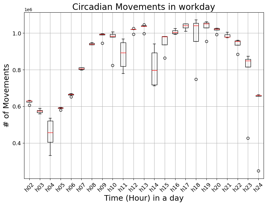
Hourly Movements

본문의 Fig. 1d 와 비슷한 플롯을 그려보았다. 본문에서는 이전 시간 대비 location의 이동이 생긴 trajectory(본문에선 trip이라 표현) 수를 계산한 것 같은데, 이 글에서 나는 해당 trajectory를 추종하는 사람들의 수(movements; a column name of ‘n’)를 더하는 방식으로 계산을 수행하였다.

MoveNum_df = defaultdict(list)
for file in DataContents[:-2]:  # Workdays Only
    MoveNum_df['Day'].append(int(file.split('-')[1]))
    temp_df = pd.read_csv(os.path.join(Temporal_BasePath, file))
    temp_df['n'] = temp_df.n.astype(np.int64)
    
    # Option 1: 경로에 0(Unknown) 이 하나라도 포함되어 있는 행은 제외
    # new_temp = temp_df[~np.any(temp_df.loc[:, temp_df.columns!='n'].values == 0, axis=1).reshape(-1, 1)].reset_index(drop=True)

    # Option 2: 경로가 모두 0(Unknown)인 행은 제외 (생각해보니 어차피 Boolean화 할때 location이 0으로 계속 안바뀌므로 False일 것이기 때문에 이 옵션은 하나마나임)
    new_temp = temp_df[~np.all(temp_df.loc[:, temp_df.columns!='n'].values == 0, axis=1).reshape(-1, 1)].reset_index(drop=True)

    # Option 3: 경로의 절반 이상이 0(Unknown)인 행은 제외
    # temp_values = temp_df.loc[:, temp_df.columns!='n'].values
    # new_temp = temp_df[~(np.sum(temp_values==0, axis=1) >= (temp_values.shape[1] / 2)).reshape(-1, 1)].reset_index(drop=True)

    # Option 4: 예외없음
    # new_temp = temp_df.copy()

    # Location ID가 바뀐 시간대 Boolean화 (바뀐 것은 True, 안바뀐 것은 False)
    MoveCheckMask = np.where(np.diff(new_temp.loc[:, new_temp.columns!='n'].values, axis=1)==0, False, True)
    for i in range(23):
        hour_key = f"h{i+2:02d}"
        total_movements = new_temp.loc[MoveCheckMask[:, i].reshape(-1, 1), 'n'].sum()
        MoveNum_df[hour_key].append(total_movements)
else:
    MoveNum_df = pd.DataFrame(MoveNum_df)

MoveNum_df

	Day	h02	h03	h04	h05	h06	h07	h08	h09	h10	...	h15	h16	h17	h18	h19	h20	h21	h22	h23	h24
0	3	606852	559901	536255	579409	652662	799121	936471	994696	993981	...	982473	1013511	1050872	1072551	1055618	1028198	978072	961790	848167	660007
1	4	623189	566318	520472	594490	671064	812592	940335	996587	978101	...	937068	994419	1050586	1054992	1063179	1022576	991314	958037	856889	660812
2	5	630087	575070	332453	592451	665917	811625	948399	945093	984020	...	863560	1003595	1040951	1041575	1050315	1025354	1005052	884543	426352	247343
3	6	629239	589552	403525	590616	666983	804797	936000	994290	1007319	...	980886	996385	1010954	954189	1029626	992259	979202	954780	874259	663403
4	7	633785	578583	457154	590369	662465	802474	945175	990851	824249	...	982211	1026021	1028607	747607	954413	1017192	974864	935576	814825	654645

5 rows × 24 columns

# Workdays Boxplot
# - box 안의 수평선은 데이터 분포의 median 지점 (50%).
# - box는 상단(75%; Q3)부터 하단(25%; Q1)까지의 데이터 범위를 말한다.
# - cap 또는 whisker(수염)은 Q3지점 이상부터 1.5 * IQR 범위내에서 가장 멀리 떨어진 데이터포인트까지 연장한 선이다. (* Q3 - Q1 = IQR(Inter Quartile Range))
# - 아래 연장선은 Q1 - 1.5 * IQR 범위 내에서 가장 멀리 떨어진 데이터 포인트까지 연장한 선
# - Circle 들은 Q3 + 1.5 * IQR 과 Q1 - 1.5 * IQR 범위에서 벗어난 일종의 Outlier(이상치)를 나타낸다.

fig, ax = plt.subplots(facecolor='w', figsize=(10,7))
MoveNum_df.loc[:, MoveNum_df.columns != 'Day'].boxplot(ax=ax, rot=45, fontsize=13, \
    color=dict(boxes='black', whiskers='black', medians='r', caps='black'))

ax.set_title("Circadian Movements in workday", fontsize=20)
ax.set_ylabel("# of Movements", fontsize=18)
ax.set_xlabel("Time (Hour) in a day", fontsize=18)
plt.show()

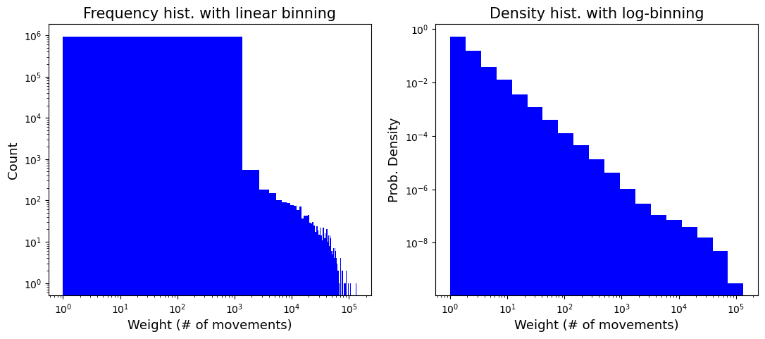
Mobility

Number of movements from location i to location j 에 대한 데이터이다. 여기서는 노드명이 Numerical ID로 표기되어 있다.
Mobility dataset은 hourly movements 들을 하나로 aggregation하였다. 즉, 해당 날을 대표하는 값들이다. (No temporal resolution)

• origin: numerical ID for each origin node;
• destination: numerical ID for each destination node;
• weight: number of movements between origin location, destination location in the day #;

본 논문에서는 3,406개 노드가 존재한다고 하지만, 모든 Day-#의 mobility 데이터셋을 열어 확인해 본 결과로는 등장하는 노드수는 2,184개가 전부이다. 아마도 movement가 없는 (weight=0) pair들, 그리고 아예 모바일 기록이 없는 기지국 Node들은 데이터셋에 포함을 안시킨 듯 하다. 논문 내용을 따라 네트워크를 구성할 땐, 1번 ~ 3406번 노드를 집어넣고 weight가 있는 것들만 대응시켜 엣지 및 weight를 올리는 식으로 작업해야할 거 같다. (세 번째 데이터셋인 ‘Distance-location.txt’에는 1번부터 3406번까지의 Node들에 대해 상대 거리가 기록되어 있다.)

Mobility_BasePath = os.path.join(BasePath, SubFiles[1])
DataContents = os.listdir(Mobility_BasePath)
print(DataContents)

['Day-3-mobility.txt', 'Day-4-mobility.txt', 'Day-5-mobility.txt', 'Day-6-mobility.txt', 'Day-7-mobility.txt', 'Day-8-mobility.txt', 'Day-9-mobility.txt']

mobility_df = []
for file in DataContents:
    mob_df = pd.read_csv(os.path.join(Mobility_BasePath, file))
    mob_df.columns = mob_df.columns.str.strip()
    mobility_df.append(mob_df)
else:
    mobility_df = pd.concat(mobility_df, ignore_index=True)

mobility_df

	origin	destination	weight
0	1	1	18530
1	2	1	2
2	4	1	5
3	5	1	15
4	6	1	1
...	...	...	...
6449644	1375	3405	1
6449645	2700	3405	1
6449646	2725	3405	1
6449647	2740	3405	1
6449648	3405	3405	5

6449649 rows × 3 columns

# 모든 mobility 데이터 기준, 존재하는 기지국 Node 갯수(unique numerical ID 갯수): 2,184개
pd.concat([mobility_df['origin'], mobility_df['destination']]).unique().shape

(2184,)

print(DataContents[0])
aday_mob = pd.read_csv(os.path.join(Mobility_BasePath, DataContents[0]))
aday_mob.columns = aday_mob.columns.str.strip() # ' destination', ' weight'로 되어있어서 보정
aday_mob

Day-3-mobility.txt

	origin	destination	weight
0	1	1	18530
1	2	1	2
2	4	1	5
3	5	1	15
4	6	1	1
...	...	...	...
937725	3403	3403	20402
937726	977	3405	1
937727	1001	3405	1
937728	2725	3405	1
937729	3405	3405	7

937730 rows × 3 columns

# Day-3-mobility에는 2,149개의 노드만 등장한다.
pd.concat([aday_mob['origin'], aday_mob['destination']]).unique().shape

(2149,)

fig, axs = plt.subplots(nrows=1, ncols=2, facecolor='w', figsize=(13, 5))
axs[0].hist(aday_mob.weight, bins=100, color='blue')
axs[0].set_ylabel("Count", fontsize=13)
axs[0].set_xlabel("Weight (# of movements)", fontsize=13)
axs[0].set_xscale('log')
axs[0].set_yscale('log')
axs[0].set_title("Frequency hist. with linear binning", fontsize=15)

axs[1].hist(aday_mob.weight, bins=np.logspace(np.log10(aday_mob.weight.min()), np.log10(aday_mob.weight.max()), 20), color='blue', density=True)
axs[1].set_ylabel("Prob. Density", fontsize=13)
axs[1].set_xlabel("Weight (# of movements)", fontsize=13)
axs[1].set_xscale('log')
axs[1].set_yscale('log')
axs[1].set_title("Density hist. with log-binning", fontsize=15)
plt.show()

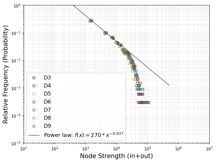
Node Strength distribution

본문의 Fig. 3를 재현해보았다. 본문에서의 Degree는 Node Strength를 말하고, Probability 는 Probability Density가 아닌 Relative Frequency (= Freq. / N_tot)의 개념인 것을 유의하자. 그리고 본문에서는 self-loop를 제외시켰는지는 모르겠지만, 이 글에서는 self-loop edge를 제외시키고 계산하였다. edge weight에는 mobility dataset의 ‘weight 컬럼’이 들어간다. 즉, number of movements인 것이다.

print(DataContents)

['Day-3-mobility.txt', 'Day-4-mobility.txt', 'Day-5-mobility.txt', 'Day-6-mobility.txt', 'Day-7-mobility.txt', 'Day-8-mobility.txt', 'Day-9-mobility.txt']

DegreeList = []
for file in DataContents:
    mob_df = pd.read_csv(os.path.join(Mobility_BasePath, file))
    mob_df.columns = mob_df.columns.str.strip()

    # Except for self-loop edges
    mob_df = mob_df[mob_df['origin'] != mob_df['destination']].reset_index(drop=True)
    
    nxG = nx.DiGraph()
    nxG.add_weighted_edges_from(zip(mob_df.origin, mob_df.destination, mob_df.weight))

    # Extract the node strength for all exisiting nodes
    degree_vals = list(dict(nxG.degree(nxG.nodes(), weight='weight')).values())
    DegreeList.append(degree_vals)

def paper_fit(x, a=270, b=-.937):
    if not isinstance(x, np.ndarray):
        x = np.array(x)
    y = a * (x ** b)
    return y

colorList = ['navy', 'darkred', 'goldenrod', 'purple', 'green', 'deepskyblue', 'saddlebrown']
fig, ax = plt.subplots(facecolor='w', figsize=(8, 6))

for i, c in enumerate(colorList):
    label = f'D{i+3}'
    linear_hist, linear_bins = np.histogram(DegreeList[i], bins=35, density=False)
    BinsCoord = [0.5 * (linear_bins[j] + linear_bins[j+1]) for j in range(len(linear_hist))]
    ax.scatter(BinsCoord, linear_hist / 3406, facecolor='None', edgecolor=c, label=label) # 본문 내용에 의하면 노드가 총 3406개인 네트워크

fit_x = np.linspace(10, 5e5, 10)
ax.plot(fit_x, paper_fit(fit_x), color='black', linewidth=.8, label=r'Power law: $f(x)=270*x^{-0.937}$')        
ax.set_yscale('log')
ax.set_xscale('log')
ax.set_ylabel('Relative Frequency (Probability)', fontsize=15)
ax.set_xlabel('Node Strength (in+out)', fontsize=15)
ax.grid(which='both', alpha=.3)
ax.set_xlim(10, 1e7)
ax.set_ylim(1e-5, 1)
ax.legend(prop={'size':13})
plt.show()

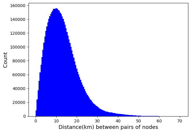
Distance-locations.txt

3,406개의 모든 기지국 사이의 (상대)거리를 수록한 데이터 파일 (단위는 km).

• origin: numerical ID for each origin node;
• destination: numerical ID for each destination node;
• distance: great-circle distance estimated by the haversine formula in kilometer between each pair of the origin location and destination location in the day #;

dist_df = pd.read_csv(os.path.join(BasePath, SubFiles[2]), header=None, names=['origin', 'destination', 'distance'])
dist_df

	origin	destination	distance
0	1	1	0.0000
1	1	2	3.3612
2	1	3	12.5690
3	1	4	2.6879
4	1	5	2.1172
...	...	...	...
11600831	3406	3402	7.6008
11600832	3406	3403	6.8099
11600833	3406	3404	11.9070
11600834	3406	3405	11.5240
11600835	3406	3406	0.0000

11600836 rows × 3 columns

NonSelf = dist_df[dist_df['origin'] != dist_df['destination']].reset_index(drop=True)
nxG = nx.Graph()
nxG.add_weighted_edges_from(zip(NonSelf.origin, NonSelf.destination, NonSelf.distance), weight='distance')
od_dist = list(nx.get_edge_attributes(nxG,'distance').values())

# No Self-loop and Undirected Graph 기준, 엣지수: (3406 * 3405) / 2 = 5,798,715개
len(od_dist)

5798715

# 기지국 Node들 사이의 상대 거리 분포 (논문에선 Heatmap으로 시각화; Fig 1-c)
# 최대 상대 거리가 70.452 km 인 기지국 pair도 있음.
# 가장 가까운 상대거리는 0.034 km
fig, ax = plt.subplots(facecolor='w', figsize=(7, 5))
ax.hist(od_dist, bins=150, color='blue')
ax.set_ylabel("Count", fontsize=13)
ax.set_xlabel("Distance(km) between pairs of nodes", fontsize=13)
plt.show()

Take-Home Message and Discussion

• 중국의 창춘시(Changchun municipality, Northeast China) 내 사람들의 모바일 데이터를 기반으로 모빌리티를 추적한 데이터를 살펴보았다.
  • Temporal Dataset / Mobility Dataset / Distance-locations.txt
  • 데이터 기간 범주는 2017년 7월 중 7일 동안(평일 5일 + 휴일 2일)을 커버하고 있다.
• Temporal Dataset을 통해 매시간마다(hourly resolution), ‘얼마나 사람들이 다른 지역으로 이동하려는 경향이 강한지’, 반대로 ‘얼마나 특정 지역에 머물러있는 경향이 강한지’ 등을 알 수 있다.
  • Temporal Dataset을 통해, 본문의 Fig.1d 와 비슷한, 평일 중 이동수(# of Movements)의 변화를 시각화해보았다.
• Mobility Dataset은 origin, destination, weight로 이뤄진 데이터이고, 여기서 weight는 od사이의 number of movements를 나타낸다.
  • Hourly movements들을 하나로 aggregation한 데이터로서, 전체 하루 동안 OD 사이 movements 수에 관한 Mobility Network를 구성할 수 있다.
  • 본문에선 3,406개의 Node가 존재한다고 하지만, 기간 전체를 통틀어 등장하는 Node는 2,184개 뿐이다. (< Notice before entering > 참고)
  • 본문의 Fig.3인 Mobility Network의 Degree(Node Strength) Distribution을 재현해보았다.
• Distance-locations.txt에는 기지국 Node들 사이의 상대거리(km)가 수록되어 있다.

fin