들어가며
Road Network & Travel Speed Dataset in Chengdu, China (aka, Megacity dataset)

들어가며

‘중국 청두시 도로망 통행속도 데이터(이하 Megacity 데이터)’를 살펴본 내용이다. 본 데이터를 알게 된 계기는 다음 논문을 읽게 되면서이다. - < Urban link travel speed dataset from a megacity road network > - Guo, Feng, et al., Scientific Data (May, 2019) - 공개 배포된 형태로 데이터셋을 전처리 및 가공하기까지 어떤 수순을 거쳤는지 논문 본문에 잘 설명이 되어 있다.

Road Network & Travel Speed Dataset in Chengdu, China (aka, Megacity dataset)

  
import os
import sys
import wget
import numpy as np
import pandas as pd
import matplotlib.pyplot as plt
import seaborn as sns
import calendar
import networkx as nx
import networkit as nk
import matplotlib.colors as mcolors
import matplotlib as mpl
import pygraphviz as pgv
import cv2
from mpl_toolkits.axes_grid1.inset_locator import inset_axes
from collections import defaultdict
from datetime import datetime
from tqdm import tqdm

Data Acquisition

Figshare: 그림, 데이터셋, 이미지 및 비디오 등을 포함한 연구 결과를 보존하고 공유하는 온라인 오픈 액세스 레포지토리

터미널 상에선, 아래 command line을 통해 데이터셋을 다운받을 수 있다.

  
>>> wget https://figshare.com/ndownloader/articles/7140209/versions/4  # 4(.zip) file download
>>> unzip 4 -d <dir_name_after_unzip>

2015.06.01 ~ 2015.07.15 사이 총 45일간의 중국 청두시의 도로망 통행 속도 데이터셋이다.
해당 기간동안, ‘5개의 대표 시간대(5 representative time horizons)’만을 다루고 있다.
- 03:00 ~ 05:00: Dawn
- 08:00 ~ 10:00: Morning
- 12:00 ~ 14:00: Noon
- 17:00 ~ 19:00: Evening
- 21:00 ~ 23:00: Night
데이터셋은 2분 단위의 기록이다. 결과적으로 하루마다 총 300개의 시간 기록(논문에선 ‘300 time periods’라 표현)이 존재한다.
각 날마다, 데이터셋은 2개의 csv 파일(_[0], _[1])로 분할하여 배포되고 있다.
- _[0].csv: 1 ~ 150 time periods
- _[1].csv: 151 ~ 300 time periods
본 도로망 통행 속도 데이터는, 해당 기간 동안, 택시 12,000대 이상으로부터 나온 30억개 이상의 GPS 궤적 데이터로부터 집계 및 추산한 결과이다.
따라서, 위 과정에서 < map matching >, < link travel speed estimation >, < data imputation > 에 대한 데이터 정제 및 전처리는 이미 되어 있다.
Megacity Dataset
- link.csv: 도로 네트워크 데이터
- speed[date]_[i].csv: 도로망 내 통행속도 데이터

  
dataset/
├── [430K]  link.csv
├── [ 23M]  speed[601]_[0].csv
├── [ 22M]  speed[601]_[1].csv
├── [ 22M]  speed[602]_[0].csv
├── ...
├── [ 23M]  speed[714]_[1].csv
├── [ 23M]  speed[715]_[0].csv
└── [ 22M]  speed[715]_[1].csv

2.0G used in 0 directories, 91 files

Road Network

“link.csv”

Attributee:
- Link: 도로링크 아이디
- Node_Start: 시작노드
- Longitude_Start, Latitude_Start: 시작노드 경위도
- Node_End: 종료노드
- Longitude_End, Latitude_End: 종료노드 경위도
- Length: 도로링크 길이(m)

  
DataPath = '/home/megacity/dataset'
DataContents = os.listdir(DataPath)
print(DataContents[0])

link.csv

  
road_network = pd.read_csv(os.path.join(DataPath, DataContents[0]))
road_network.head(5)

	Link	Node_Start	Longitude_Start	Latitude_Start	Node_End	Longitude_End	Latitude_End	Length
0	1	0	103.946006	30.750660	48	103.956494	30.745080	1179.207157
1	2	0	103.946006	30.750660	64	103.941276	30.754493	620.905375
2	3	0	103.946006	30.750660	16	103.952551	30.756752	921.041014
3	4	1	104.062539	30.739077	1288	104.062071	30.732501	730.287581
4	5	1	104.062539	30.739077	311	104.060024	30.742693	467.552294

Geographical visualization

  
NodeList = pd.concat([road_network['Node_Start'], road_network['Node_End']], ignore_index=True).unique()
fig, ax = plt.subplots(facecolor='w', figsize=(8,8))
for row in tqdm(road_network.iloc):
    link_loc = row[['Longitude_Start', 'Longitude_End', 'Latitude_Start', 'Latitude_End']].values
    x, y = link_loc[:2], link_loc[2:]
    ax.plot(x, y, marker='o', markerfacecolor='w', ms=0.7, color='black', linewidth=.4)

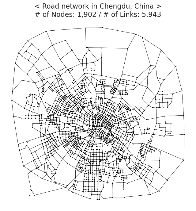
title = f"< Road network in Chengdu, China >\n# of Nodes: {NodeList.shape[0]:,} / # of Links: {road_network.shape[0]:,}"
ax.set_title(title, fontsize=16)
ax.axis('off')
plt.show()

5943it [00:05, 1048.30it/s]

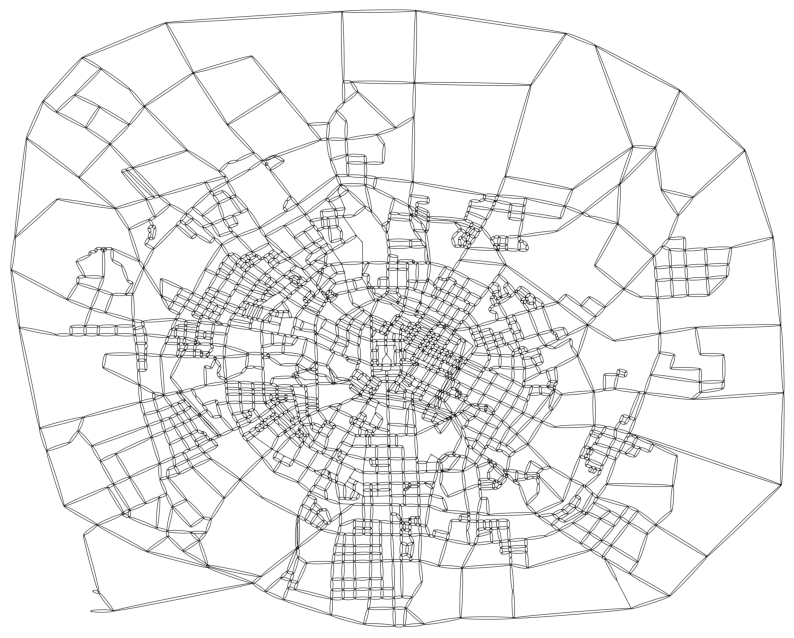
Network visualization

  
# Make a dictionary containing real-world coordinates of nodes
node_pos_dict = defaultdict(list)
for node in tqdm(road_network['Node_Start'].unique()):
    lon, lat = road_network[road_network.Node_Start==node][['Longitude_Start', 'Latitude_Start']].values[0]
    if len(node_pos_dict[node]) == 0:
        node_pos_dict[node] = [lon, lat]

for node in tqdm(road_network['Node_End'].unique()):
    lon, lat = road_network[road_network.Node_Start==node][['Longitude_End', 'Latitude_End']].values[0]
    if len(node_pos_dict[node]) == 0:
        node_pos_dict[node] = [lon, lat]

print(f"The total number of nodes: {len(node_pos_dict.keys()):,}")

100%|██████████| 1902/1902 [00:01<00:00, 1559.17it/s]
100%|██████████| 1902/1902 [00:01<00:00, 1583.15it/s]

The total number of nodes: 1,902

  
megaNetG = nx.MultiDiGraph()
megaNetG.add_edges_from(zip(road_network.Node_Start, road_network.Node_End))

# Create a graph object for Graphviz
agraph = nx.nx_agraph.to_agraph(megaNetG)

# For Graphviz, set the node positions, node_size, label as none.
# If wanting to adjust the size of node, 'fixedsize' attribute of node must be 'True' (** important !!)
# Note that setting the values of width / height / arrowsize / Graphviz scale is under some trial-error.
for node in agraph.nodes():
    node.attr['pos'] = '{},{}'.format(node_pos_dict[int(node)][0], node_pos_dict[int(node)][1])
    node.attr['fixedsize'] = True
    node.attr['width'] = '0.07'
    node.attr['height'] = '0.07'
    node.attr['label'] = ''

for edge in agraph.edges():
    edge.attr['arrowsize'] = '0.3'
    edge.attr['penwidth'] = '2.5'

# Draw the graph using Graphviz
agraph.graph_attr.update(scale='15000')

# forcing to my_position of nodes, rather than 'neato' layout.
agraph.draw('megacity_road_network.png', prog='neato', args='-n')

# Show the plot
fig, ax = plt.subplots(facecolor='w', figsize=(10,10))
img = plt.imread('megacity_road_network.png')
ax.imshow(img)
ax.axis('off')
plt.show()

Link Travel Speed

“speed[date]_[i].csv”

Attributee:
- Period: 통행 속도 시점대
- Link: 도로링크
- Speed: 해당 도로링크의 통행 속도

  
print(DataContents[1])

    speed[601]_[0].csv

  
origin_mega = pd.read_csv(os.path.join(DataPath, DataContents[1]))

# 150개의 시점(time periods) * 5943개의 도로링크 = 891,450개의 rows
print(origin_mega)

                 Period  Link      Speed
    0       03:00-03:02     1  31.769048
    1       03:00-03:02     2  49.450000
    2       03:00-03:02     3  42.780000
    3       03:00-03:02     4  35.150000
    4       03:00-03:02     5  25.950000
    ...             ...   ...        ...
    891445  12:58-13:00  5939  22.030769
    891446  12:58-13:00  5940  25.875000
    891447  12:58-13:00  5941  20.572917
    891448  12:58-13:00  5942  43.980000
    891449  12:58-13:00  5943  16.480000
    
    [891450 rows x 3 columns]

Personal renewal idea

데이터셋 하나로 전부 다루고 싶어서 개인적으로 해보는 전처리 (다시 말해서, 따라할 필요없음)

날짜 컬럼 추가 (dtype: int64).
- ex) 1 June -> 601
요일 컬럼 추가 (dtype: str).
- ex) 1 June -> ‘Mon’
기존의 ‘Period’ 컬럼 이름을 ‘time’으로 변경, 그리고 시작 시점을 기준으로 단순화 (dtype: int64).
- ex) 03:00 ~ 03:02 » 300
time 컬럼 기반, 시간대 컬럼 추가 (dtype: str).
- ex) 300 ~ 458 time: ‘Dawn’, 800 ~ 958: ‘Morn’, 1200 ~ 1358: ‘Noon’, 1700 ~ 1858: ‘Even’, 2100 ~ 2258: ‘Night’
하루 기준, 시간 순서 컬럼 추가 (dtype: int64). (논문 내 ‘time periods’에 해당하는 값)
- ex) ‘time’ 컬럼의 {300, 302, 304, …, 2354, 2356, 2358} 에 대응하는 {1,2,3, …, 298, 299, 300}
45일 간의 모든 데이터 하나의 .pkl로 저장 (~ 3.3 GB)
Checkpoints during this renewal
- Checkpoint_1: check if the size of each dataset is 891,450.
- Checkpoint_2: check if the number of road links is 5,943.
- Checkpoint_3: check if each of 5,943 road links has 150 time moments.

  
assign_horizon = lambda t: 'Dawn' if 300 <= t < 500 else \
         'Morn' if 800 <= t < 1000 else \
         'Noon' if 1200 <= t < 1400 else \
         'Even' if 1700 <= t < 1900 else \
         'Night' if 2100 <= t < 2300 else \
         'wtf'
         
time_seq = [[],[]]
for i in range(2):
    for seq in range(1+(i*150), 151+(i*150)):
        for _ in range(5943):
            time_seq[i].append(seq)

mega_dataset = pd.DataFrame()
for filename in tqdm(DataContents[1:]):
    ZeroOne = int(filename.split(']')[1].split('[')[1])
    mon_date = [int(filename.split(']')[0].split('[')[1])]
    ymd = f"2015{mon_date[0]:04d}"
    day = [calendar.day_name[datetime.strptime(ymd, '%Y%m%d').weekday()][:3]]
    one_mega = pd.read_csv(os.path.join(DataPath, filename))
    if (one_mega.shape[0]!=891450) | (one_mega.groupby('Link').ngroups!=5943): # Checkpoint_1 + Checkpoint_2
        error_msg = f"Strange dataset detected: {filename}"
        print(error_msg)
        print(''.ljust(len(error_msg), '-'))
        continue

    one_mega['mon_date'] = pd.Series(mon_date*891450)
    one_mega['day'] = pd.Series(day*891450)
    one_mega['time'] = one_mega['Period'].apply(lambda x: int(''.join(x.split('-')[0].split(':'))))
    one_mega['Period'] = one_mega['time'].apply(assign_horizon)
    if not np.array_equal(one_mega.value_counts('time').values, [5943]*150): # Checkpoint_3
        error_msg = f"Not all links have 150 time_moments: {filename}"
        print(error_msg)
        print(''.ljust(len(error_msg), '-'))
        continue

    one_mega = one_mega.sort_values(by='time').reset_index(drop=True)
    one_mega['time_seq'] = pd.Series(time_seq[ZeroOne])
    mega_dataset = pd.concat([mega_dataset, one_mega], ignore_index=True)

mega_dataset.to_pickle("my_megacity_dataset_20150601_to_0715.pkl")

One Megacity Dataset

“my_megacity_dataset_20150601_to_0715.pkl”

Attributee:
- Period: 시간대 (Dawn, Morn, Noon, Even, Night)
- Link: 도로링크
- Speed: 해당 도로링크의 통행 속도
- mon_date: 날짜 및 일자
- day: 요일
- time: 시간 시점
- time_seq: 하루 기준 몇 번째 기록인지, [1~300]

  
mega_dataset = "my_megacity_dataset_20150601_to_0715.pkl"
mega_dataset = pd.read_pickle(os.path.join('/home/megacity/', mega_dataset))
mega_dataset

	Period	Link	Speed	mon_date	day	time	time_seq
0	Dawn	1	31.769048	601	Mon	300	1
1	Dawn	3968	43.550000	601	Mon	300	1
2	Dawn	3967	45.350000	601	Mon	300	1
3	Dawn	3966	28.141667	601	Mon	300	1
4	Dawn	3965	31.450000	601	Mon	300	1
...	...	...	...	...	...	...	...
80230495	Night	1977	44.825000	715	Wed	2258	300
80230496	Night	1976	23.857669	715	Wed	2258	300
80230497	Night	1975	19.990186	715	Wed	2258	300
80230498	Night	1984	60.830769	715	Wed	2258	300
80230499	Night	5943	15.381818	715	Wed	2258	300

80230500 rows × 7 columns

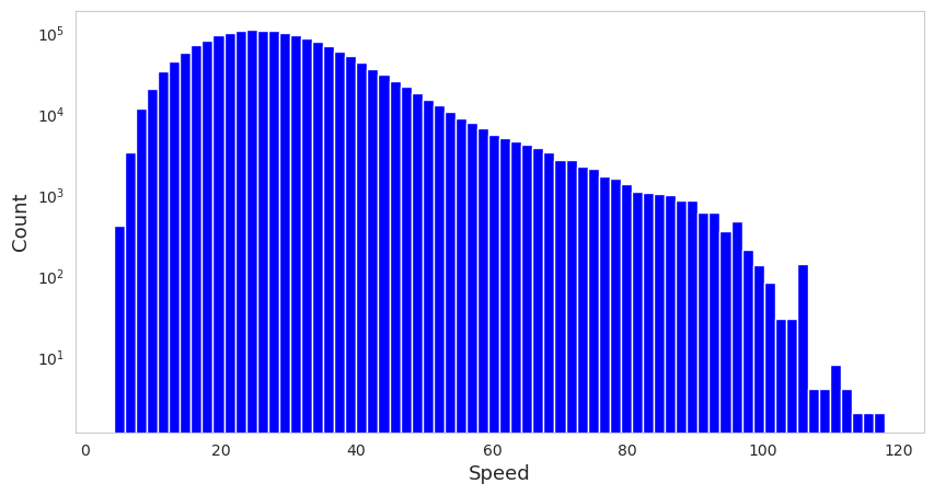
Daily analysis

2015년 6월 1일, 평일
하루 전체 속도 통계 분포, 아침 시간대 공간 분포를 알아본다.

  
aday_mega_dataset = mega_dataset[mega_dataset['mon_date']==601].reset_index(drop=True)

  
fig, ax = plt.subplots(facecolor='w', figsize=(10,5))
aday_mega_dataset['Speed'].hist(bins=70, color='blue', ax=ax)
print(f"Minimum speed: {aday_mega_dataset['Speed'].min()}, Maximum speed: {aday_mega_dataset['Speed'].max()}")
print(f"Average speed: {aday_mega_dataset['Speed'].mean()}")
ax.grid(visible=False)
ax.set_yscale('log')
ax.set_ylabel("Count", fontsize=13)
ax.set_xlabel("Speed", fontsize=13)
plt.show()


    Minimum speed: 4.2, Maximum speed: 117.98
    Average speed: 29.466771318855514

  
cmap = mpl.colors.LinearSegmentedColormap.from_list("", ["red", "yellow", "green", "blue"])
# Based on the distribution of traffic speed in daily, Normalization for a given color map.
norm = mpl.colors.Normalize(aday_mega_dataset['Speed'].min(), aday_mega_dataset['Speed'].max())

def create_meganet_agraph(meganet):
    megaNetG = nx.MultiDiGraph()
    megaNetG.add_edges_from(zip(meganet.Node_Start, meganet.Node_End))
    agraph = nx.nx_agraph.to_agraph(megaNetG)
    for node in agraph.nodes():
        node.attr['pos'] = '{},{}'.format(node_pos_dict[int(node)][0], node_pos_dict[int(node)][1])
        node.attr['fixedsize'] = True
        node.attr['width'] = '0.07'
        node.attr['height'] = '0.07'
        node.attr['label'] = ''

    for edge in agraph.edges():
        edge.attr['arrowsize'] = '0.3'
        edge.attr['penwidth'] = '5.5'

    # Draw the graph using Graphviz
    agraph.graph_attr.update(scale='15000')
    return agraph

def save_edgecolor_agraph(agraph_obj, link_speed_df, cmap, norm, prefix='', savepath=False):
    '''
        This function is only managing the edge colors 
        in terms of link_travel_speed 
        based on the predefined <cmap> and <norm>.
    '''
    for edge in agraph_obj.edges():
        node_st, node_ed = edge
        edge_speed = link_speed_df[(link_speed_df['Node_Start']==int(node_st)) & (link_speed_df['Node_End']==int(node_ed))]['Speed'].values[0]
        edge.attr['color'] = mpl.colors.to_hex(cmap(norm(edge_speed)))

    file_name = prefix + 'EdgeColor_megaroad_network.png'
    if savepath is not False:
        saving_file = os.path.join(savepath, file_name)
    else:
        saving_file = os.path.join(os.getcwd(), file_name)
    agraph_obj.draw(saving_file, prog='neato', args='-n')
    return saving_file

  
morn_aday_dataset = aday_mega_dataset[aday_mega_dataset['Period']=='Morn'].reset_index(drop=True)
morn_aday_dataset = pd.merge(morn_aday_dataset, road_network[['Link', 'Node_Start', 'Node_End']], on='Link')
# 2015년 6월 1일, 아침 8시
snap_morn_aday = morn_aday_dataset[morn_aday_dataset['time']==800].reset_index(drop=True)

  
agraph_obj = create_meganet_agraph(road_network)
saved_location = save_edgecolor_agraph(agraph_obj, snap_morn_aday, cmap=cmap, norm=norm)
print(saved_location)

fig, ax = plt.subplots(facecolor='w', figsize=(10, 10))

sm = plt.cm.ScalarMappable(cmap=cmap, norm=norm)
sm.set_array([])
cbaxes = inset_axes(ax, width="99%", height="1.5%", bbox_to_anchor=(0,0.08,1,1), bbox_transform=ax.transAxes, loc='upper left') 
c_bar = fig.colorbar(sm, cax=cbaxes, orientation='horizontal')

img = plt.imread(saved_location)
ax.imshow(img)
ax.axis('off')
year_mon_date = datetime.strptime(f"{snap_morn_aday['mon_date'].values[0]:04d}", "%m%d").strftime("2015-%m-%d")
hour_min = datetime.strptime(f"{snap_morn_aday['time'].values[0]:04d}", '%H%M').strftime("%H:%M")
fig_title = f"{hour_min} in Chengdu, China ({year_mon_date}, Morning)\nLink Travel Speed on road network"
fig.suptitle(fig_title, fontsize=15, y=0.9)
plt.show()


    /home/megacity/megacity_gitlab/EdgeColor_megaroad_network.png

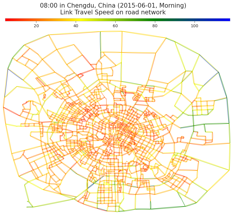
An circadian change for spatial distribution of link travel speed

2015년 6월 1일, 평일
Ultimately, we produce a video displaying the circadian change for spatial distribution.

  
# 2015-06-01 (Monday)
for one_period in ['Dawn', 'Noon', 'Even', 'Night']:
    oneper_aday_dataset = aday_mega_dataset[aday_mega_dataset['Period']==one_period].reset_index(drop=True)
    oneper_aday_dataset = pd.merge(oneper_aday_dataset, road_network[['Link', 'Node_Start', 'Node_End']], on='Link')
    for i, time in tqdm(enumerate(oneper_aday_dataset['time'].unique())):
        snap_oneper_aday = oneper_aday_dataset[oneper_aday_dataset['time']==time].reset_index(drop=True)
        if i == 0:
            print("Initially generate an object of agraph...")
            period = snap_oneper_aday['Period'].values[0]
            period = period + 'ing' if period == 'Morn' else period
            agraph_obj = create_meganet_agraph(road_network)

        snap_filename = save_edgecolor_agraph(agraph_obj, snap_oneper_aday, cmap=cmap, norm=norm, prefix=f'{i}_', savepath='/home/megacity/debris_img')
        
        fig, ax = plt.subplots(facecolor='w', figsize=(10,10))
        
        sm = plt.cm.ScalarMappable(cmap=cmap, norm=norm)
        sm.set_array([])
        cbaxes = inset_axes(ax, width="99%", height="1.5%", bbox_to_anchor=(0,0.08,1,1), bbox_transform=ax.transAxes, loc='upper left') 
        c_bar = fig.colorbar(sm, cax=cbaxes, orientation='horizontal')

        img = plt.imread(snap_filename)
        ax.imshow(img)
        ax.axis('off')

        year_mon_date = datetime.strptime(f"{snap_oneper_aday['mon_date'].values[0]:04d}", "%m%d").strftime("2015-%m-%d")
        hour_min = datetime.strptime(f"{snap_oneper_aday['time'].values[0]:04d}", '%H%M').strftime("%H:%M")
        fig_title = f"{hour_min} in Chengdu, China ({year_mon_date}, {period})\nLink Travel Speed on road network"
        fig.suptitle(fig_title, fontsize=15, y=0.9)

        new_savepath = "/home/megacity/main_img"
        new_savefile = f"{i}_{year_mon_date}_{snap_oneper_aday['Period'].values[0]}_travelspeed.png"
        plt.savefig(os.path.join(new_savepath, new_savefile), dpi=200, pad_inches=.2, bbox_inches='tight')
        plt.close()

  
# 5-periods Convergence and Text on 'img' read by cv2.imread()
img_folder = '/home/megacity/main_img'

font = cv2.FONT_HERSHEY_COMPLEX # font
fontScale = 2.5 # fontScale
color = (0, 0, 0) # black color (Note that cv2 is handling the color as BGR code)
thickness = 7 # Text thickness

concat_images = []
text_index = []
dummy_image_num = 10
period_range = {
    'Dawn': '03:00 ~ 05:00', 
    'Morn': '08:00 ~ 10:00', 
    'Noon': '12:00 ~ 14:00', 
    'Even': '17:00 ~ 19:00', 
    'Night': '21:00 ~ 23:00'
}
Periods = ['Dawn', 'Morn', 'Noon', 'Even', 'Night']
for i, one_period in enumerate(Periods):
    images = [img for img in os.listdir(img_folder) if one_period in img]
    images.sort(key=lambda x: int(x.split('_')[0]))
    # total_images_num = len(images)
    extend_images = [images[0]] * dummy_image_num
    extend_images.extend(images)
    total_images_num = len(extend_images)
    concat_images.extend(extend_images)
    text_index.extend([idx + (i * total_images_num) for idx in range(dummy_image_num)])

else:
    video_name = "20150601_aday_withText_travelspeed.mp4"
    frame = cv2.imread(os.path.join(img_folder, concat_images[0]))
    height, width, layers = frame.shape
    Codec = cv2.VideoWriter_fourcc(*'mp4v')
    video = cv2.VideoWriter(video_name, Codec, 5, (width, height)) # frame 은 len(concat_images)와 딱맞게 떨어져야 함. 
    for i, img in enumerate(concat_images):
        im = cv2.imread(os.path.join(img_folder, img), cv2.COLOR_BGR2RGB)

        text_repos_indicator = -1
        if i in text_index:
            Periods_indicator = i // total_images_num
            text_period_img = Periods[Periods_indicator]
            time_range = period_range[text_period_img]
            text_period_img = text_period_img + 'ing' if text_period_img == 'Morn' else text_period_img
            text_period_img += f':: {time_range}'

            if text_repos_indicator != Periods_indicator: # i == 0
                text_size, _ = cv2.getTextSize(text_period_img, font, fontScale, thickness)
                text_x = int((width - text_size[0]) / 2)
                text_y = int((height - text_size[1]) / 2)
                text_repos_indicator = Periods_indicator

            im = cv2.putText(im, f'{text_period_img}', (text_x, text_y), font, fontScale, color, thickness, cv2.LINE_AA)
        video.write(im)

    video.release()
    cv2.destroyAllWindows()

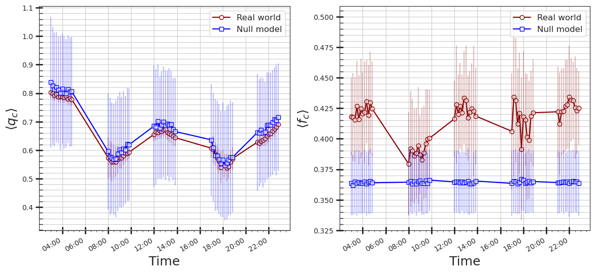
Employing ‘Percolation Approach’

Based on [Li, Daqing, et al. “Percolation transition in dynamical traffic network with evolving critical bottlenecks.” Proceedings of the National Academy of Sciences 112.3 (2015)]
Converts ‘Link Travel Speed’ to ‘Link quality (q)’.

\[q_{ij}(t) = \frac{v_{ij}(t)}{v^{95th}_{ij}}\]

  
grouped_mega = mega_dataset.groupby(by=['mon_date', 'Link'])
maximal_df = grouped_mega['Speed'].apply(lambda x: np.percentile(x, 95)).reset_index(name='maximal')
concat_mega = pd.merge(mega_dataset, maximal_df, on=['mon_date', 'Link'])
concat_mega['q'] = concat_mega[['Speed', 'maximal']].apply(lambda x: round(x[0] / x[1], 4), axis=1)

for mondate in tqdm(concat_mega['mon_date'].unique()):
    aday_temp = concat_mega[concat_mega['mon_date']==mondate].reset_index(drop=True)
    filename = f"2015{mondate:04d}_qRatio_megacity.pkl"
    aday_temp.to_pickle(filename)

  
# Percolation 결과는 별도의 작업 공간에서 계산 후 가져옴.
qcfcPath = '/home/megacity/qcfc'
qcfc_DataContents = os.listdir(qcfcPath)
qcfc_dataset = pd.DataFrame()
qcfc_rand_dataset = pd.DataFrame()
for filename in qcfc_DataContents:
    if 'RANDOM' not in filename:
        temp = pd.read_pickle(os.path.join(qcfcPath, filename))
        qcfc_dataset = pd.concat([qcfc_dataset, temp], ignore_index=True)
    else:
        temp = pd.read_pickle(os.path.join(qcfcPath, filename))
        qcfc_rand_dataset = pd.concat([qcfc_rand_dataset, temp], ignore_index=True)

  
sns.set_style('white', {'axes.linewidth': 0.5})
plt.rcParams['xtick.major.size'] = 20
plt.rcParams['xtick.major.width'] = 4
plt.rcParams['xtick.bottom'] = True
plt.rcParams['ytick.left'] = True

  
workday_qcfc = qcfc_dataset[qcfc_dataset['day'].isin(['Mon', 'Tue', 'Wed', 'Thu', 'Fri'])].reset_index(drop=True)
dayoff_qcfc = qcfc_dataset[qcfc_dataset['day'].isin(['Sat', 'Sun'])].reset_index(drop=True)
workday_rand_qcfc = qcfc_rand_dataset[qcfc_rand_dataset['day'].isin(['Mon', 'Tue', 'Wed', 'Thu', 'Fri'])].reset_index(drop=True)

  
fmt = mpl.dates.DateFormatter('%H:%M')

workday_grouped = workday_qcfc.groupby(by='time')
workday_rand_grouped = workday_rand_qcfc.groupby(by='time')

mean_qc = workday_grouped['q_c'].mean().reset_index()['q_c']
std_qc = workday_grouped['q_c'].agg(np.std, ddof=0).reset_index()['q_c']
mean_fc = workday_grouped['f_c'].mean().reset_index()['f_c']
std_fc = workday_grouped['f_c'].agg(np.std, ddof=0).reset_index()['f_c']
time_xaxis = list(map(lambda x: datetime.strptime(f'{x:04d}', '%H%M') , workday_grouped['q_c'].mean().index))

mean_rand_qc = workday_rand_grouped['q_c'].mean().reset_index()['q_c']
std_rand_qc = workday_rand_grouped['q_c'].agg(np.std, ddof=0).reset_index()['q_c']
mean_rand_fc = workday_rand_grouped['f_c'].mean().reset_index()['f_c']
std_rand_fc = workday_rand_grouped['f_c'].agg(np.std, ddof=0).reset_index()['f_c']

fig, axs = plt.subplots(ncols=2, facecolor='w', figsize=(14, 6.5))
axs[0].plot(time_xaxis, mean_qc, c='darkred', marker='o', markerfacecolor='w', label='Real world')
axs[0].errorbar(time_xaxis, mean_qc, yerr=std_qc, color='darkred', alpha=.25)
axs[0].plot(time_xaxis, mean_rand_qc, c='blue', marker='s', markerfacecolor='w', label='Null model')
axs[0].errorbar(time_xaxis, mean_rand_qc, yerr=std_rand_qc, color='blue', alpha=.25)
axs[0].xaxis.set_major_formatter(fmt)
axs[0].minorticks_on()
axs[0].tick_params(which='major', length=10, width=2, direction='inout')
axs[0].tick_params(which='minor', length=5, width=1, direction='in', axis='y')
axs[0].grid(which='minor', axis='y')
axs[0].grid(which='major', axis='both')
axs[0].legend(prop={'size':12})
axs[0].set_ylabel(r"$\langle q_{c} \rangle$", fontsize=18)
axs[0].set_xlabel("Time", fontsize=18)

axs[1].plot(time_xaxis, mean_fc, c='darkred', marker='o', markerfacecolor='w', label='Real world')
axs[1].errorbar(time_xaxis, mean_fc, yerr=std_fc, color='darkred', alpha=.25)
axs[1].plot(time_xaxis, mean_rand_fc, c='blue', marker='s', markerfacecolor='w', label='Null model')
axs[1].errorbar(time_xaxis, mean_rand_fc, yerr=std_rand_fc, color='blue', alpha=.25)
axs[1].xaxis.set_major_formatter(fmt)
axs[1].minorticks_on()
axs[1].tick_params(which='major', length=10, width=2, direction='inout')
axs[1].tick_params(which='minor', length=5, width=1, direction='in', axis='y')
axs[1].grid(which='minor', axis='y')
axs[1].grid(which='major', axis='both')
axs[1].legend(prop={'size':12})
axs[1].set_ylabel(r"$\langle f_{c} \rangle$", fontsize=18)
axs[1].set_xlabel("Time", fontsize=18)

fig.autofmt_xdate()
plt.show()

Take-Home Message and Discussion

중국 청두시의 도로망에 대해 총 45일 간의 통행속도 데이터셋을 들여다 보았다.
figshare 온라인 공유 저장소에서 데이터셋을 배포하고 있다. (본 작업은 개인 workspace에 해당 데이터를 내려받아 사용)
데이터의 출처인 ‘Guo, Feng, et al., 2019’ 논문의 연구팀이 데이터 정제를 깔끔하게 잘 해놓아서 결측값(Missing value)이 없다.
본 작업에서 다룬 중국 청두시 도로 네트워크의 크기는 서울시 topis로부터 제공받은 데이터 내 ‘서울시 도로 네트워크 크기’와 비슷하다.

fin

중국 청두시 도로망 및 속도 데이터 분석