들어가며
지난 주 Batista e Silva, et al. (2020) 논문을 읽다가 또 기록해둘만 한 데이터를 발견했다. 바로 2011년 EU 28개국(영국의 브렉시트로 현재는 27개국)의 Population 데이터이다. 지난 포스트에서 다룬 WorldPop 데이터는 거의 모든 개별 국가의 2000년부터 2020년 사이의 Population 기록들을 커버하고 있지만, 이번 EU Population 데이터는 2011년 한 해에 집중한 대신 월별(Monthly)로 되어 있다.
해당 데이터는 European Commission(유럽연합 집행위윈회) 내부의 Joint Research Centre(JRC; 공동연구센터)에서 공공 배포하는 여러 데이터 중 하나다. JRC는 유럽연합(EU)의 정책 의사결정 지원과 동시에 독립적으로 과학기술 자문 업무를 수행하는 기관인데, 그 과정에서 여러 프로젝트 과제의 부산물 또는 그 결과물들을 공적으로 배포하는 것 같다. 아무튼 이번 글에선 < ENACT-POP R2020A > 란 프로젝트의 EU-28 2011 Population Grid 데이터를 들여다 보기로 한다.
데이터에 대한 상세한 내부 설명은 다음 링크의 pdf 파일을 참고하자.
2011 Monthly EU Population
1
2
3
4
5
6
7
8
9
10
| import os
import numpy as np, pandas as pd, geopandas as gpd
import matplotlib as mpl, matplotlib.pyplot as plt
from mpl_toolkits.axes_grid1.inset_locator import inset_axes
from osgeo import gdal
import folium
from folium.elements import Figure
# raster data 읽을 떄, 쓸만한 또 다른 모듈.
import rasterio
|
Understanding of GIS terminologies
Coordinate Reference System(CRS; 또는 SRS: Spatial Reference System)는 지구 표면 상의 위치를 표현 및 정의하기 위한 일련의 규칙들을 묶어놓은 집합이다.
A4 용지 위에 놓여있는 동전의 위치를 2개의 좌표로 친구한테 설명해야하는 상황이라 해보자.
그 친구는 오로지 당신의 설명만을 듣고, 본인이 가진 또 다른 A4 용지에다가 그 동전의 위치를 정확히 그려내는 것이 목표다.
이를 위해, 당신은 아래와 같은 ‘나만의 좌표 시스템’을 만들어 친구에게 소개해주고자 한다.
- 자 우선, A4 용지를… 용지의 짧은 쪽이 위로 향하게 두고 설명할거야.
- 이 때 용지의 가장 왼쪽 아래 모서리 귀퉁이를 2차원 x, y의 (0, 0) 지점이라 하자.
- 그리고 오른쪽과 위쪽 방향이 각각 +x, +y 이라 하자.
- 마지막으로… 여기 내 x, y 좌표계의 단위는 자로 쟀을 때의 1cm와 동일해.
여기까지 설명해주면, 이제 끝이다. 예컨대 친구한테 이제 “동전의 위치는 (x, y) = (1.5, 2) 위치에 있어.” 라고 설명해주면, 친구는 본인의 A4 용지에다가 동전의 위치를 정확히 찍어낼 수 있다.
지구 표면 상의 위치를 표현하는 과정도 대충 이런 상황과 비슷한거다. 다만, 지구는 3차원 물체이고 그 표면은 곡면을 가진다는 차이가 있다. 이런 물체 상에 표시된 지점을 설명하려면, 우선 (위 예시의) A4 용지처럼 동일한 형태(size, shape)의 지구 모형을 누구든지 동일하게 떠올릴 수 있어야 한다. 이 개념이 GIS 용어로 자주 등장하는 Reference ellipsoid이다. 이 Reference ellipsoid (or Earth ellipsoid)는 Semi-major axis with meter / Semi-minor axis with meter / Flattening factor 로 그 크기와 형태가 정의된 지구 타원체 모형을 의미한다. 시대 흐름에 따라 또는 필요에 따라 다양한 종류의 타원체 모형이 존재하는데, 대표적으로 Bessel 1841, Clarke 1866, GRS 1980, WGS 1984 같은 것들이 있다.
그러면 이제 동일한 타원체 모형만 모두가 들고 있으면 되냐. 아니다. 마지막으로 타원체 모형의 중심점과 표면을 지구와 어떻게 일치 시킬건 지에 대한 정의도 필요하다. 이 내용까지 포함하면, 비로소 GIS의 (Horizontal) Datum 이란 개념까지 도달하는 것이다. 즉, Datum은 Reference Ellipsoid 개념을 포함하는 상위 개념이다. 대표적으로 많이 쓰이는 Datum으로는 ETRS89, WGS84, NAD83 같은 것들이 있다.
이제 타원체 모형의 형태를 지구에 빗대어 정확히 일치시켰다. 하지만 아직 그 표면엔 아무 것도 그려져 있지 않은 백지일 뿐이다. 공간 내 특정 지점을 어떤 값으로 표현하기 위해선 좌표 체계를 갖춰야한다. 다시 말해, Coordinate system; CS을 얹혀야 한다. 이 좌표 체계는 원점이 어디인지 / 각 단위는 Datum 기반에서 축척(scale)이 얼마인지 등의 내용을 포함하고 있다. 대표적인 CS type으로는 (longitude, latitude)로 표현되는 Geographic Coordinate System(GCS), (x, y)로 표현되는 Projected Coordinate System(PCS) 타입이 있다. 여기서 PCS 형태의 좌표계는 구좌표계에서 Conversion (~ Projection)하여 얻게 되는 2차원 공간 상의 좌표계이다. 따라서 각기 다른 Map Projection 방법들을 통해 나온 다양한 PCS 좌표계들이 존재한다.
즉, 서두에서 말한 지구 표면 상의 위치를 표현 및 정의하기 위한 일련의 규칙들로서, Reference Ellipsoid / Datum / Coordinate System (+ Projection Type)들의 조합으로 이루어진 집합을 CRS 라고 하는 것이다.
막상 GIS 일부 용어들의 개념을 정확히 공부할 겸 작성을 시작했는 데, 생각보다 만만치 않았다…
이제와서 생각해보면, 그럴만 한게 ‘지도’ 자체의 역사만 두고 봐도 기원전까지 거슬러 올라가고, 심지어는 완전히 spherical하지도 ellipsoidal하지도 않은 3차원 지구의 표면을 2차원으로 최대한 정확히 투영시켜 표현한다는 행위 자체가 상당히 challenging 한 문제이자 어찌보면 극복할 수 없는 한계일테니 말이다. 수 세기동안 얼마나 많은 기하학적 개념들과 방법론들이 투입되고 시도되었을까. 애초에 이에 관한 모든 개념을 반나절, 하루이틀 만에 완전히 이해하려는 것 자체가 자만이라는 생각이 든다. 용어의 개념들을 하나하나 정리하며 깊게 파고들수록 한 분야안에서도 끝도 없이 이어져 나온다. 아무튼 여기저기서 읽은 내용들과 머릿 속에 나름대로 정리한 내용들을 이렇게 기록해 남겨둔다.
Data Overview and Data Acquisition
오늘 살펴볼 2011 EU-28 Monthly Population 데이터셋은 다음 jrc의 데이터 열린광장 사이트(?)에서 직접 내려받을 수 있다.
데이터셋은 데이터 위치를 어떤 CRS 체계로 표현된 건 지에 따라 크게 “ETRS89 (Datum)”과 “WGS84 (Datum)” 으로 나뉜다. 그리고 각 CRS 종류마다 Day-time(주간; 낮)과 Night-time(야간; 밤) 시간대에 관한 데이터가 있다. 아쉽게도 Day-time & Night-time이 정확히 몇시부터 몇시 사이인 건지는 알아낼 수 없었다.
1
2
3
4
5
6
7
8
9
10
11
12
13
14
15
16
17
18
19
20
21
| ./eupop_dataset
├── [761M] ETRS89
│ ├── [223M] day_time
│ │ ├── [ 15M] ENACT_POP_D012011_EU28_R2020A_3035_1K_V1_0.tif
│ │ ├── ...
│ │ └── [ 15M] ENACT_POP_D122011_EU28_R2020A_3035_1K_V1_0.tif
│ └── [156M] night_time
│ ├── [ 10M] ENACT_POP_N012011_EU28_R2020A_3035_1K_V1_0.tif
│ ├── ...
│ └── [ 10M] ENACT_POP_N122011_EU28_R2020A_3035_1K_V1_0.tif
│
└── [1.9G] WGS84
├── [539M] day_time
│ ├── [ 37M] ENACT_POP_D012011_EU28_R2020A_4326_30ss_V1_0.tif
│ ├── ...
│ └── [ 37M] ENACT_POP_D122011_EU28_R2020A_4326_30ss_V1_0.tif
└── [496M] night_time
├── [ 34M] ENACT_POP_N012011_EU28_R2020A_4326_30ss_V1_0.tif
├── ...
└── [ 34M] ENACT_POP_N122011_EU28_R2020A_4326_30ss_V1_0.tif
|
1
2
| BasePath = './eupop_dataset'
print(os.listdir(BasePath))
|
1
2
3
4
5
6
7
8
9
10
11
12
13
14
15
16
17
18
19
20
21
22
23
24
25
26
27
28
29
30
| def AboutTif(tif):
'''
Tiff or Tif 데이터를 로드한 gdal object에 대해 기본적인 정보를 보여주는 함수
'''
num_bands = tif.RasterCount
msg = f"※ Number of bands: {num_bands}"
print(msg)
print(''.ljust(len(msg), '-'))
rows, cols = tif.RasterYSize, tif.RasterXSize
msg = f"※ Raster size: {rows} rows x {cols} columns"
print(msg)
print(''.ljust(len(msg), '-'))
desc = tif.GetDescription()
msg = f'Raster description: {desc}'
print(msg)
print(''.ljust(len(msg), '-'))
for bandnum in range(1, num_bands+1):
bandmsg = f" For {bandnum} band "
print(f"{bandmsg:+^{len(msg)}}")
band = tif.GetRasterBand(bandnum)
null_val = band.GetNoDataValue()
print(f"Null value: {null_val}") # " 아, 여긴 확실히 없다. "는 곳을 나타내는 값.
minimum, maximum, mean, sd = band.GetStatistics(True, True)
print(f"Mean: {mean:.3f} / SD: {sd:.3f} / min: {minimum:.3f} / max: {maximum:.3f}")
print(''.ljust(len(msg), '+'), end='\n\n' if num_bands!=1 else '\n')
|
Notice before entering
동일한 Month / time-period 더라도, 어느 CRS (ETRS89 or WGS84)인지에 따라 raster size와 statistics가 차이가 있다.
1
2
3
4
5
6
7
8
| crs_types = os.listdir(BasePath)
for crs in crs_types:
msg = f'< {crs} >'
print(f'{msg:=^100}')
crsPath = os.path.join(BasePath, crs, 'day_time')
tf = gdal.Open(os.path.join(crsPath, os.listdir(crsPath)[0]))
AboutTif(tf)
print()
|
1
2
3
4
5
6
7
8
9
10
11
12
13
14
15
16
17
18
19
20
21
22
23
| =============================================< ETRS89 >=============================================
※ Number of bands: 1
--------------------
※ Raster size: 4367 rows x 5585 columns
---------------------------------------
Raster description: ./eupop_dataset/ETRS89/day_time/ENACT_POP_D012011_EU28_R2020A_3035_1K_V1_0.tif
--------------------------------------------------------------------------------------------------
+++++++++++++++++++++++++++++++++++++++++++ For 1 band +++++++++++++++++++++++++++++++++++++++++++
Null value: -200.0
Mean: 91.223 / SD: 646.370 / min: 0.000 / max: 59130.750
++++++++++++++++++++++++++++++++++++++++++++++++++++++++++++++++++++++++++++++++++++++++++++++++++
=============================================< WGS84 >==============================================
※ Number of bands: 1
--------------------
※ Raster size: 5535 rows x 13467 columns
----------------------------------------
Raster description: ./eupop_dataset/WGS84/day_time/ENACT_POP_D022011_EU28_R2020A_4326_30ss_V1_0.tif
---------------------------------------------------------------------------------------------------
+++++++++++++++++++++++++++++++++++++++++++ For 1 band ++++++++++++++++++++++++++++++++++++++++++++
Null value: -200.0
Mean: 48.776 / SD: 377.934 / min: 0.000 / max: 44234.873
+++++++++++++++++++++++++++++++++++++++++++++++++++++++++++++++++++++++++++++++++++++++++++++++++++
|
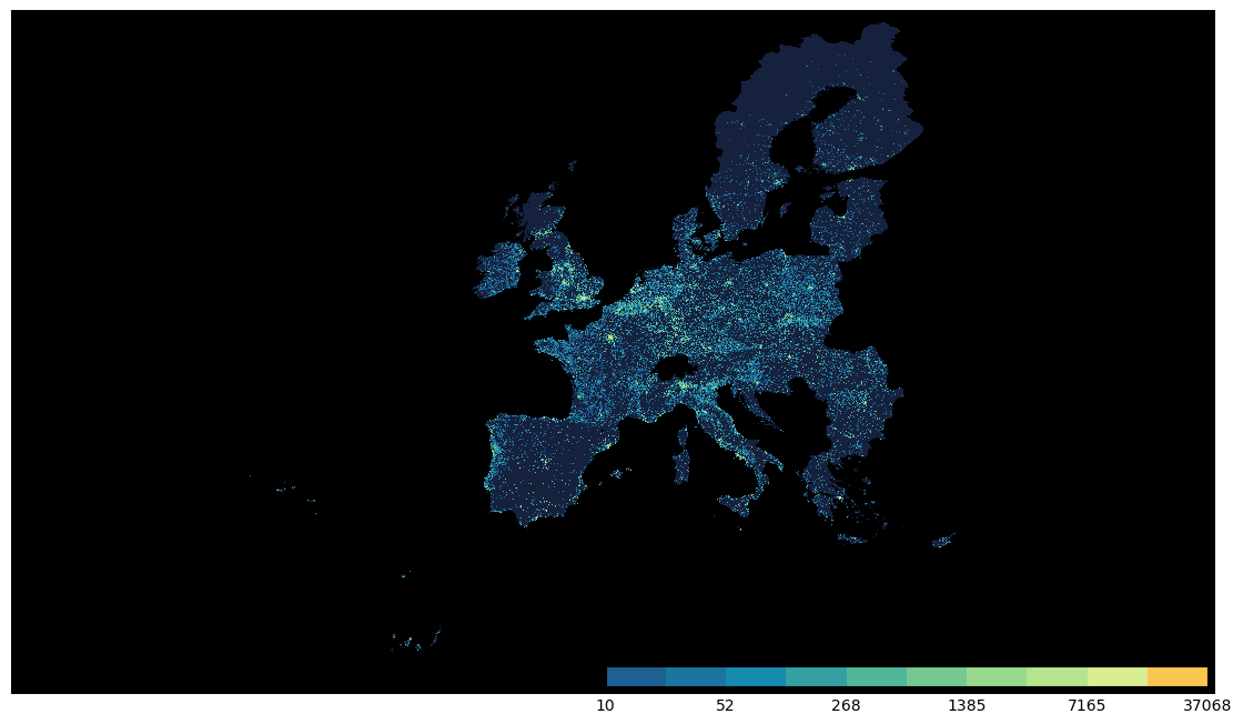
EU Population Dataset
본 글에서는 우리에게 친숙한 좌표계 longitude, latitude 단위인 GCS 좌표계를 활용하는 WGS84 데이터를 기준으로 설명한다.
1
| BasePath = './eupop_dataset/WGS84'
|
1
2
3
4
5
6
7
8
9
10
11
12
13
14
15
16
17
18
| DataPath = os.path.join(BasePath, 'day_time')
Tifs = []
daytime_temp = []
for file in os.listdir(DataPath):
if not file.endswith('.tif'):
continue
daytime_temp.append(gdal.Open(os.path.join(DataPath, file)))
else:
Tifs.append(daytime_temp)
DataPath = os.path.join(BasePath, 'night_time')
nighttime_temp = []
for file in os.listdir(DataPath):
if not file.endswith('.tif'):
continue
nighttime_temp.append(gdal.Open(os.path.join(DataPath, file)))
else:
Tifs.append(nighttime_temp)
|
1
2
| target_tf = Tifs[1][0]
AboutTif(target_tf)
|
1
2
3
4
5
6
7
8
9
10
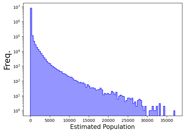
| ※ Number of bands: 1
--------------------
※ Raster size: 5535 rows x 13467 columns
----------------------------------------
Raster description: ./eupop_dataset/WGS84/night_time/ENACT_POP_N012011_EU28_R2020A_4326_30ss_V1_0.tif
-----------------------------------------------------------------------------------------------------
++++++++++++++++++++++++++++++++++++++++++++ For 1 band +++++++++++++++++++++++++++++++++++++++++++++
Null value: -200.0
Mean: 59.726 / SD: 400.093 / min: 0.000 / max: 37067.639
+++++++++++++++++++++++++++++++++++++++++++++++++++++++++++++++++++++++++++++++++++++++++++++++++++++
|
1
2
3
4
5
| band_data = target_tf.GetRasterBand(1)
null_val = band_data.GetNoDataValue()
img = band_data.ReadAsArray()
band_val = img.flatten()
band_val = band_val[band_val!=null_val]
|
1
2
3
4
5
6
| fig, ax = plt.subplots(facecolor='w', figsize=(7, 5))
ax.hist(band_val, bins=100, color='blue', histtype='step', hatch='///////')
ax.set_yscale('log')
ax.set_xlabel("Estimated Population", fontsize=15)
ax.set_ylabel('Freq.', fontsize=20)
plt.show()
|
1
2
3
4
5
6
7
8
9
10
| # Understanding cmap and norm
cList = ["#1e6091", "#1a759f", "#168aad", "#34a0a4", "#52b69a", "#76c893", "#99d98c", "#b5e48c", "#d9ed92", "#f9c74f"]
cmap = mpl.colors.LinearSegmentedColormap.from_list("", cList, len(cList))
logbounds = np.logspace(np.log10(10), np.log10(band_val.max()), len(cList)+1) # Note that I freely selected the value range for visualization.
print(f"bins = {len(np.diff(logbounds))}")
norm = mpl.colors.BoundaryNorm(logbounds, len(cList))
cmap.set_under('black')
cmap.set_bad(color='#16213E')
cmap.set_over(color='red')
cmap
|
1
2
3
4
5
6
7
8
9
10
11
12
13
| # set the color as a bad(np.nan) color in colorbar
img[np.logical_and(img >= 0, img <= 10)] = np.nan
fig, ax = plt.subplots(facecolor='w', figsize=(14, 8))
# aspect의 디폴트값은 equal임. 입력된 array 크기로 figure가 forcing 됨.
im = ax.imshow(img, cmap=cmap, norm=norm, interpolation='none', aspect='auto')
ax.axis('off')
cb_ax = inset_axes(ax, width="50%", height="3%", loc='lower right')
fig.colorbar(im, cax=cb_ax, orientation='horizontal')
plt.show()
|
Interactive Map with folium
1
2
3
4
5
6
7
8
9
10
11
12
13
14
15
16
17
18
19
| # Get coordinates, cols and rows
geotransform = target_tf.GetGeoTransform()
# Get extent
xmin = geotransform[0]
ymax = geotransform[3]
xmax = xmin + geotransform[1] * target_tf.RasterXSize
ymin = ymax + geotransform[5] * target_tf.RasterYSize
print(xmin, ymin, xmax, ymax)
# Get Central point
center_x = (xmin + xmax) / 2
center_y = (ymin + ymax) / 2
# Raster convert to array in numpy
band_data = target_tf.GetRasterBand(1)
null_val = band_data.GetNoDataValue()
img = band_data.ReadAsArray()
img[np.logical_or(img == null_val, img < 10)] = 0
|
1
| -53.51028043444351 24.790983341916238 58.714719116656504 70.91598315741624
|
1
2
3
4
5
6
| def folium_get_color(origin_v, norm, cmap):
if origin_v >= 10:
r, g, b, _ = cmap(norm(origin_v))
return (r, g, b, 0.7)
else:
return (1, 1, 1, 0) # white & transparent
|
1
2
3
4
5
6
7
8
9
10
11
12
| # Visualization in folium
v_min, v_max = img.min(), img.max()
fm = folium.Map(location=[center_y, center_x], zoom_start=4, prefer_canvas=True, tiles='cartodbpositron')
# opacity로 전체 컬러 알파 조절
fm_layer = folium.raster_layers.ImageOverlay(image=img, bounds=[[ymin, xmin], [ymax, xmax]], opacity=0.7, mercator_project=True, colormap=lambda x: folium_get_color(x, norm, cmap))
fm_layer.add_to(fm)
fig = Figure(width=1200, height=600)
fig.add_child(fm)
fm.save('folium_map_PreferCanvas_Opacity0_7.html')
|
1
| <folium.raster_layers.ImageOverlay at 0x2b782743b250>
|
folium을 통해 interactive map 에 맵핑시킨 결과는 여기 클릭을 통해 열람해볼 수 있다. 불러오는 데 시간이 좀 걸릴 수 있음.
본 시각화에 활용한 데이터는 WGS84/night_time/ENACT_POP_N012011_EU28_R2020A_4326_30ss_V1_0.tif 이다.
Please note that… 포스팅 이후로 시간이 좀 지난 시점이면 url access가 안될 수도 있음.
fin