들어가며
지금까지 많은 연구들은 기후적 요소(climatic driver; 기온/강수/습도/구름/바람)의 변화들이 우리 인간 사회에 끼치는 영향들을 ‘재해로 인한 경제적 손실’ 같은 지표로 정량화하고 이에 대응해왔다.
하지만 자연 재해 리스크에 대한 더욱 정확한 이해와 대응력을 갖추기 위해서는, 비기후적 요소(non-climatic driver)들의 변화 역시 함께 주시하고 파악하여 계산과 대응에 반영할 필요가 있다.
예컨대 특정 지역에 대해, 거주하는 인구수나 경제적 생산가치, 유형적 재산(부동산 건물, 인프라 등)의 크기 등을 고려했을 때, 노출된 규모가 크다면 우리들은 해당 지역의 재해 대책 마련에 대한 예산을 더욱 투입하여 재난 피해를 최소화해야할 것이다. 즉 다시 말해, 재난 위험에 노출된 사회경제적인 요소 수준이 어느 정도인지 정확한 진단들을 보유하고 있어야 한다는 이야기다. 이러한 요소들을 Socio-economic Exposures라고 부른다.
토지의 특성도 여러 가지 측면에서 기술할 수 있겠지만, 대표적으로 토지의 다짐도 (soil compaction; soil sealing degree)를 떠올려 볼 수 있다. 토지는 토지 이용의 목적에 따라 절토/성토/정지/포장되어 그 형질이 변화된다. 이러한 과정에 따라 토지 속 공극비가 조절되고 토지의 압축성이 변화한다. 만약 압축성이 작은 토지 위에 비가 내려 빗물이 쌓인다면, 물은 토양에 흡수되어 지하수를 통해 바다로 배출될 것이다. 하지만 압축성이 큰 토지 형질의 경우, 빗물은 흡수되기보단 토지 위에 그대로 쌓이는 비중이 많아져 홍수 피해 (floods)란 재난 리스크를 유발하게 된다. 즉, 이 경우 토지의 다짐도 수준이 floods’ hazard (위험요소)로 인식된다는 이야기다. 그리고 보통 도시나 개발 지역의 토지 다짐도 수준이 높다.
정리하자면, 과거 역사적 재난의 크기와 또는 그로 인한 경험적 피해 규모들로 오늘 날의 기후 변화로 인한 영향을 평가하고 가늠하는 것은 한계가 있다. 왜냐하면, 시대가 흐르면서 함께 변화하는 socio-economic exposure 요소들과 토지 형질 따위의 환경의 변화 때문이다. 즉, 앞서 언급한 사회경제적 요소들이 특정 지역에 얼마나 노출되어 있는지/토지의 특징은 어떠한지 함께 고려해야, 가까운 미래의 우리 사회에 끼칠 기후적 영향들을 제대로 파악하고 대응할 수 있는 것이다.
이러한 취지로 이번에 읽어본 논문의 연구팀은 지난 2018년에 Hanze v1.0 모델을 시작으로 올 2023년 6월 Hanze v2.0 모델을 소개하는 논문을 내었고, Hanze v2.0 모델에서 추출된 1870년부터 2020년 사이 유럽 내 socio-economic exposures와 토지 이용 및 특징 (Land Cover/use and Soil sealing degree)에 관한 데이터들을 오픈 배포하였다. 데이터셋들의 validation 과정과 결과는 본문을 참조하면 된다. 이제 데이터셋들을 하나하나 열어 살펴보자.
Hanze v2.0 European Exposure Estimates
References
- Paprotny, D., & Mengel, M. (2023). Population, land use and economic exposure estimates for Europe at 100 m resolution from 1870 to 2020. Scientific Data, 10(1), 372.
- Paprotny, D. (2023). Pan-European exposure maps and uncertainty estimates from HANZE v2.0 model, 1870-2020.
- Paprotny, D. (2023). HANZE v2.0 exposure model.
1
2
3
4
5
6
7
8
9
10
11
12
13
14
import os
import numpy as np, pandas as pd, matplotlib as mpl, matplotlib.pyplot as plt
from mpl_toolkits.axes_grid1.anchored_artists import AnchoredSizeBar
from matplotlib.patches import Rectangle
from mpl_toolkits.axes_grid1.inset_locator import inset_axes
from PIL import Image
import cv2
from osgeo import gdal
from tqdm import tqdm
import warnings

# mpl.use('module://matplotlib_inline.backend_inline')
warnings.simplefilter(action='ignore', category=FutureWarning)
os.environ['GDAL_PAM_ENABLED'] = 'NO'
osgeo.gdal installation
일반적으론 conda install -c conda-forge gdal 또는 pip install GDAL 로 간편하게 설치할 수 있다고 하는데, 내 경우엔 solving environment 에서 stuck (being hung forever…) 되는 현상이 발생했고 후자의 방법에선 bashrc와 libgdal config를 다시 잘 설정하라는 성가신 요구가 주어졌다. 그래서 찾은 대안이 mamba 라는 아나콘다(Anaconda.com) 팀에서 conda를 c++ 버전으로 re-implementation한 새로운 패키지 매니저를 이용하는 것이다. 사실 앞서 이야기한 solving environment forever 외에도 고질적인 문제들이 많았는데 그런 것들을 이번 mamba에선 잘 (특히 속도 및 안정성면에서) 개선했다고 한다. 그리고 무엇보다 그냥 기존 conda “command line”에 conda대신 mamba만 바꿔 넣으면 되는 식이라 (= high backward compatibility) 원래 conda를 쓰던 사용자면 더욱이 안 쓸 이유가 없는 것 같다.
아무튼 아래대로 진행하면 GDAL python package를 문제없이 내 conda env에다가 설치할 수 있다.
1
2
>>> conda install -c conda-forge mamba  # mamba package manager installation
>>> mamba install -c gdal-master gdal
Data Acquisition and Data Tree
전체 데이터셋은 May 2, 2023 Zenodo 링크에서 내려받을 수 있다. 압축 파일들의 크기를 제외하면 본 데이터셋 전체 크기는 약 30GB 정도 된다.
데이터의 Spatial Coverage는 유럽 내 NUT3 지역들이다.
NUTS: Nomenclature of Units for Territorial Statistics (통계지역단위명명법). NUTS는 유럽연합(EU)에서 최초로 정의했고, 주로 유럽연합 회원국들에서 사용하는 범유럽 내 행정지역 구분단위이다.
총 3-level hierarchy (NUTS1, NUTS2, NUTS3) 를 가지고 있고, 숫자가 클 수록 구역들을 더욱 세밀하게 구분한 것이라고 보면 된다.
데이터셋 종류
- Raster Dataset (.tif; temporal coverage: 1870년 ~ 2020년)
- CLC: land cover/use dataset - CLC라는 토지이용 분류법으로 특정 grid가 어느 토지목적 및 용도인지 기록한 데이터.
- Imperviousness density(%): 해당 지역 및 토지의 불침투성(imperviousness)을 수치화한 데이터. (e.g. 불침투성이 높은 지역은 우천시 비가 토양에 스며들지않고 표면에 쌓여서 범람이나 홍수 피해의 위험이 있다.)
- GDP: 해당 grid의 GDP 수준이 어느 정도 되는지 기록한 데이터. (2020년 기준 Euro 단위)
- Fixed Asset(FA): 해당 grid 내에 유형적 재산(부동산 및 건물 등)의 규모가 어느 정도인지 기록한 데이터. (2020년 기준 Euro 단위)
- Population: 거주하는 인구가 얼마나 되는지.
- METADATA-1: Land_cover_use_legend
- A list of labels for each CLC/GRID_CODE
- METADATA-2: Exposure_(coastal/river)_hazard_zone.csv
- Uncertainty estimates of exposure
- METADATA-3: NUTS3database(economy/population_land_use).xlsx
- Subnational and national-level statistical data on population, land use and economic variables.
1
2
3
4
5
6
7
8
9
10
11
12
13
14
15
16
17
18
19
20
21
22
23
24
25
26
27
28
29
30
31
32
33
34
35
36
37
38
39
40
41
42
43
44
45
46
47
48
49
50
51
>>> tree --du -h

dataset/
├── [1.6M]  Exposure_coastal_hazard_zone.csv
├── [5.2M]  Exposure_river_hazard_zone.csv
├── [4.0M]  NUTS3_database_economy.xlsx
├── [3.0M]  NUTS3_database_population_land_use.xlsx
│
├── [9.0G]  Fixed_asset_value_1870_2020
│   ├── [195M]  FA_100m_1870.tif
│   ├── [197M]  FA_100m_1880.tif
│   ├── ...
│   └── [258M]  FA_100m_2020.tif
│
├── [ 10G]  GDP_1870_2020
│   ├── [232M]  GDP_100m_1870.tif
│   ├── [233M]  GDP_100m_1880.tif
│   ├── ...
│   └── [289M]  GDP_100m_2020.tif
│
├── [3.1G]  Imperviousness_1870_2020
│   ├── [ 67M]  Imp_1870.tif
│   ├── [ 69M]  Imp_1880.tif
│   ├── ...
│   └── [ 87M]  Imp_2020.tif
│
├── [4.2G]  Land_cover_use_1870_2020
│   ├── [106M]  CLC_1870.tif
│   ├── [106M]  CLC_1880.tif
│   ├── ...
│   └── [112M]  CLC_2020.tif
│
├── [3.5G]  Population_1870_2020
│   ├── [ 84M]  Population_100m_1870.tif
│   ├── [ 85M]  Population_100m_1880.tif
│   ├── ...
│   └── [ 95M]  Population_100m_2020.tif
│
├── [ 46K]  Land_cover_use_legend
│   ├── [ 16K]  Land_cover_use_classes.xlsx
│   ├── [ 16K]  clc_legend_arcgis_raster.tif.lyr
│   └── [ 14K]  clc_legend_qgis_raster.qml
└── [ 23G]  zipfile
    ├── [7.0G]  Fixed_asset_value_1870_2020.zip
    ├── [8.5G]  GDP_1870_2020.zip
    ├── [2.1G]  Imperviousness_1870_2020.zip
    ├── [3.4G]  Land_cover_use_1870_2020.zip
    ├── [ 20K]  Land_cover_use_legend.zip
    └── [2.2G]  Population_1870_2020.zip

  53G used in 7 directories, 209 files
1
2
3
4
5
6
7
8
9
10
11
12
13
14
BasePath = 'dataset/'
subDirs = []
BaseFiles = []
for content in os.listdir(BasePath):
    if os.path.isfile(os.path.join(BasePath, content)):
        BaseFiles.append(content)
    else:
        subDirs.append(content)

print("Files on the base path:")
print(BaseFiles)
print()
print("Sub-directories:")
print(subDirs)
1
2
3
4
5
Files on the base path:
['Exposure_coastal_hazard_zone.csv', 'Exposure_river_hazard_zone.csv', 'NUTS3_database_economy.xlsx', 'NUTS3_database_population_land_use.xlsx']

Sub-directories:
['Fixed_asset_value_1870_2020', 'GDP_1870_2020', 'Imperviousness_1870_2020', 'Land_cover_use_1870_2020', 'Land_cover_use_legend', 'Population_1870_2020', 'zipfile']
1
2
3
4
5
6
7
8
9
10
11
12
13
14
15
16
17
18
19
20
21
22
23
24
25
26
27
28
29
30
31
def AboutTif(tif):
    '''
        Tiff or Tif 데이터를 로드한 gdal object에 대해 기본적인 정보를 보여주는 함수
    '''
    num_bands = tif.RasterCount
    msg = f"※ Number of bands: {num_bands}"
    print(msg)
    print(''.ljust(len(msg), '-'))

    rows, cols = tif.RasterYSize, tif.RasterXSize
    msg = f"※ Raster size: {rows} rows x {cols} columns"
    print(msg)
    print(''.ljust(len(msg), '-'))

    desc = tif.GetDescription()
    msg = f'Raster description: {desc}'
    print(msg)
    print(''.ljust(len(msg), '-'))

    for bandnum in range(1, num_bands+1):
        bandmsg = f" For {bandnum} band "
        print(f"{bandmsg:+^{len(msg)}}")

        band = tif.GetRasterBand(bandnum)
        null_val = band.GetNoDataValue()
        print(f"Null value: {null_val}") # " 아, 여긴 확실히 없다. "는 곳을 나타내는 값.

        minimum, maximum, mean, sd = band.GetStatistics(False, True) # first argument 를 True로 두면, Approximate한 값을 리턴한다.
        print(f"Mean: {mean:.3f} / SD: {sd:.3f} / min: {minimum:.3f} / max: {maximum:.3f}")
        print(''.ljust(len(msg), '+'), end='\n\n' if num_bands!=1 else '\n')
CLC: Land cover/use dataset
CLC(Corine Land Cover) classification
Needed directories:
- dataset/Land_cover_use_1870_2020
- dataset/Land_cover_use_legend
CLC Classes
1
2
3
print(f"Contents in a directory of < {subDirs[-3]} >")
clc_legend_files = os.listdir(os.path.join(BasePath, subDirs[-3]))
clc_legend_files
1
2
3
4
5
Contents in a directory of < Land_cover_use_legend >

['clc_legend_arcgis_raster.tif.lyr',
 'clc_legend_qgis_raster.qml',
 'Land_cover_use_classes.xlsx']
1
pd.read_excel(os.path.join(BasePath, subDirs[-3], clc_legend_files[-1]), engine='openpyxl')
| GRID_CODE | CLC_CODE | LABEL1 | LABEL2 | LABEL3 | |
|---|---|---|---|---|---|
| 0 | 1 | 111 | Artificial surfaces | Urban fabric | Continuous urban fabric |
| 1 | 2 | 112 | Artificial surfaces | Urban fabric | Discontinuous urban fabric |
| 2 | 3 | 121 | Artificial surfaces | Industrial, commercial and transport units | Industrial or commercial units |
| 3 | 4 | 122 | Artificial surfaces | Industrial, commercial and transport units | Road and rail networks and associated land |
| 4 | 5 | 123 | Artificial surfaces | Industrial, commercial and transport units | Port areas |
| 5 | 6 | 124 | Artificial surfaces | Industrial, commercial and transport units | Airports |
| 6 | 7 | 131 | Artificial surfaces | Mine, dump and construction sites | Mineral extraction sites |
| 7 | 8 | 132 | Artificial surfaces | Mine, dump and construction sites | Dump sites |
| 8 | 9 | 133 | Artificial surfaces | Mine, dump and construction sites | Construction sites |
| 9 | 10 | 141 | Artificial surfaces | Artificial, non-agricultural vegetated areas | Green urban areas |
| 10 | 11 | 142 | Artificial surfaces | Artificial, non-agricultural vegetated areas | Sport and leisure facilities |
| 11 | 12 | 211 | Agricultural areas | Arable land | Non-irrigated arable land |
| 12 | 13 | 212 | Agricultural areas | Arable land | Permanently irrigated land |
| 13 | 14 | 213 | Agricultural areas | Arable land | Rice fields |
| 14 | 15 | 221 | Agricultural areas | Permanent crops | Vineyards |
| 15 | 16 | 222 | Agricultural areas | Permanent crops | Fruit trees and berry plantations |
| 16 | 17 | 223 | Agricultural areas | Permanent crops | Olive groves |
| 17 | 18 | 231 | Agricultural areas | Pastures | Pastures |
| 18 | 19 | 241 | Agricultural areas | Heterogeneous agricultural areas | Annual crops associated with permanent crops |
| 19 | 20 | 242 | Agricultural areas | Heterogeneous agricultural areas | Complex cultivation patterns |
| 20 | 21 | 243 | Agricultural areas | Heterogeneous agricultural areas | Land principally occupied by agriculture, with... |
| 21 | 22 | 244 | Agricultural areas | Heterogeneous agricultural areas | Agro-forestry areas |
| 22 | 23 | 311 | Forest and semi natural areas | Forests | Broad-leaved forest |
| 23 | 24 | 312 | Forest and semi natural areas | Forests | Coniferous forest |
| 24 | 25 | 313 | Forest and semi natural areas | Forests | Mixed forest |
| 25 | 26 | 321 | Forest and semi natural areas | Scrub and/or herbaceous vegetation associations | Natural grasslands |
| 26 | 27 | 322 | Forest and semi natural areas | Scrub and/or herbaceous vegetation associations | Moors and heathland |
| 27 | 28 | 323 | Forest and semi natural areas | Scrub and/or herbaceous vegetation associations | Sclerophyllous vegetation |
| 28 | 29 | 324 | Forest and semi natural areas | Scrub and/or herbaceous vegetation associations | Transitional woodland-shrub |
| 29 | 30 | 331 | Forest and semi natural areas | Open spaces with little or no vegetation | Beaches, dunes, sands |
| 30 | 31 | 332 | Forest and semi natural areas | Open spaces with little or no vegetation | Bare rocks |
| 31 | 32 | 333 | Forest and semi natural areas | Open spaces with little or no vegetation | Sparsely vegetated areas |
| 32 | 33 | 334 | Forest and semi natural areas | Open spaces with little or no vegetation | Burnt areas |
| 33 | 34 | 335 | Forest and semi natural areas | Open spaces with little or no vegetation | Glaciers and perpetual snow |
| 34 | 35 | 411 | Wetlands | Inland wetlands | Inland marshes |
| 35 | 36 | 412 | Wetlands | Inland wetlands | Peat bogs |
| 36 | 37 | 421 | Wetlands | Maritime wetlands | Salt marshes |
| 37 | 38 | 422 | Wetlands | Maritime wetlands | Salines |
| 38 | 39 | 423 | Wetlands | Maritime wetlands | Intertidal flats |
| 39 | 40 | 511 | Water bodies | Inland waters | Water courses |
| 40 | 41 | 512 | Water bodies | Inland waters | Water bodies |
| 41 | 42 | 521 | Water bodies | Marine waters | Coastal lagoons |
| 42 | 43 | 522 | Water bodies | Marine waters | Estuaries |
| 43 | 44 | 523 | Water bodies | Marine waters | Sea and ocean |
| 44 | 48 | 999 | NODATA | NODATA | NODATA |
CLC Dataset
1
subDirs
1
2
3
4
5
6
7
['Fixed_asset_value_1870_2020',
 'GDP_1870_2020',
 'Imperviousness_1870_2020',
 'Land_cover_use_1870_2020',
 'Land_cover_use_legend',
 'Population_1870_2020',
 'zipfile']
1
2
3
clcPath = os.path.join(BasePath, 'Land_cover_use_1870_2020')
clcContents = os.listdir(clcPath)
print(clcContents)
1
['CLC_1870.tif', 'CLC_1880.tif', 'CLC_1890.tif', 'CLC_1900.tif', 'CLC_1910.tif', 'CLC_1920.tif', 'CLC_1930.tif', 'CLC_1940.tif', 'CLC_1950.tif', 'CLC_1955.tif', 'CLC_1960.tif', 'CLC_1965.tif', 'CLC_1970.tif', 'CLC_1975.tif', 'CLC_1980.tif', 'CLC_1985.tif', 'CLC_1990.tif', 'CLC_1995.tif', 'CLC_2000.tif', 'CLC_2001.tif', 'CLC_2002.tif', 'CLC_2003.tif', 'CLC_2004.tif', 'CLC_2005.tif', 'CLC_2006.tif', 'CLC_2007.tif', 'CLC_2008.tif', 'CLC_2009.tif', 'CLC_2010.tif', 'CLC_2011.tif', 'CLC_2012.tif', 'CLC_2013.tif', 'CLC_2014.tif', 'CLC_2015.tif', 'CLC_2016.tif', 'CLC_2017.tif', 'CLC_2018.tif', 'CLC_2019.tif', 'CLC_2020.tif']
1
2
3
# Open CLC_2020.tif
clc_sample = gdal.Open(os.path.join(clcPath, clcContents[-1]))
clc_sample
1
<osgeo.gdal.Dataset; proxy of <Swig Object of type 'GDALDatasetShadow *' at 0x2ad836ac5110> >
1
AboutTif(clc_sample)
1
2
3
4
5
6
7
8
9
10
※ Number of bands: 1
--------------------
※ Raster size: 40300 rows x 38686 columns
-----------------------------------------
Raster description: dataset/Land_cover_use_1870_2020/CLC_2020.tif
-----------------------------------------------------------------
++++++++++++++++++++++++++ For 1 band +++++++++++++++++++++++++++
Null value: -128.0
Mean: 6.763 / SD: 10.793 / min: 0.000 / max: 48.000
+++++++++++++++++++++++++++++++++++++++++++++++++++++++++++++++++
1
2
band_data = clc_sample.GetRasterBand(1)
band_arr = band_data.ReadAsArray()
1
2
3
uni_val, counts = np.unique(band_arr.flatten(), return_counts=True)
uni_cnt_dict = dict(zip(uni_val, counts))
print(uni_cnt_dict)
1
{0: 1054655295, 1: 651457, 2: 16185621, 3: 2930798, 4: 391522, 5: 111500, 6: 314723, 7: 657085, 8: 117835, 9: 87857, 10: 316907, 11: 1237019, 12: 108962574, 13: 3939701, 14: 659855, 15: 3868078, 16: 2847839, 17: 4734889, 18: 41248948, 19: 540747, 20: 19870168, 21: 19736734, 22: 3306310, 23: 55153419, 24: 76809465, 25: 27558595, 26: 12633870, 27: 17511216, 28: 9830303, 29: 22554254, 30: 658536, 31: 6944318, 32: 13930342, 34: 1582250, 35: 1202907, 36: 11614310, 37: 413399, 38: 56733, 39: 18663, 40: 1232769, 41: 11655801, 42: 242107, 43: 49525, 44: 19471, 48: 85}
1
2
3
4
5
6
7
8
# Understanding cmap and norm
cList = ["paleturquoise", "red", "sandybrown", "lime", "green", "olive", "silver", "slategrey", "cyan"]
cmap = mpl.colors.LinearSegmentedColormap.from_list("", cList, len(cList))
cBounds = [0, 1, 12, 18, 23, 26, 30, 35, 40, 45]
norm = mpl.colors.BoundaryNorm(cBounds, len(cList))
cmap.set_under('aqua')
# cmap.set_bad(color='#16213E')
cmap.set_over(color='white')
1
2
3
4
5
6
7
8
9
10
11
12
13
14
15
16
17
18
19
20
21
22
23
24
25
26
27
28
29
30
31
32
33
34
35
36
37
38
39
40
41
42
43
44
45
46
47
48
49
50
51
52
53
54
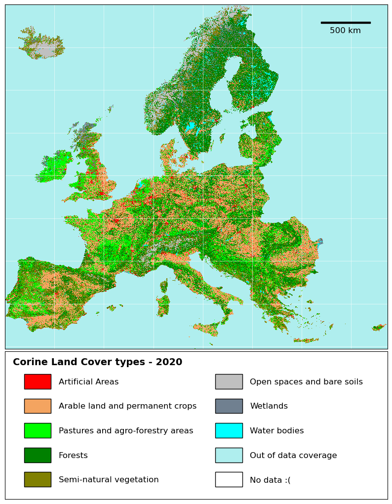
fig, axs = plt.subplots(nrows=2, ncols=1, facecolor='w', figsize=(10, 13), height_ratios=[3.5, 1.5])
## CLC tif map Axis
axs[0].imshow(band_arr, cmap=cmap, norm=norm, interpolation='None', aspect='auto')
scale_bar = AnchoredSizeBar(axs[0].transData, 5000, '500 km', 'upper right', \
fontproperties={'size':12}, sep=5, borderpad=2, \
size_vertical=200, frameon=False, color='black')
axs[0].add_artist(scale_bar)
axs[0].grid(color='white', alpha=.7, linewidth=.6)
axs[0].set_xticklabels([])
axs[0].set_yticklabels([])
axs[0].tick_params(tick1On=False)
## Colors Desc. Axis
axs[1].set_xlim(0, 1)
axs[1].set_ylim(0, 1)
color_label = {'olive': 'Semi-natural vegetation', \
'green': 'Forests', \
'lime': 'Pastures and agro-forestry areas', \
'sandybrown': 'Arable land and permanent crops', \
'red': 'Artificial Areas', \
'white': 'No data :(', \
'paleturquoise': 'Out of data coverage', \
'cyan': 'Water bodies', \
'slategrey': 'Wetlands', \
'silver': 'Open spaces and bare soils'
}
cl_list = list(color_label.items())
cl_idx = 0 # initialize color and label index
x, init_y = 0.05, round(1/12, 3) # initial y_position and stepper; 동일한 높이의 color box가 총 12개 있다 침.
for init_x in [0, 0.5]:
for y_th in range(5): # 한 축에 다섯개씩
color, label = cl_list[cl_idx]
c_x, c_y = init_x + x, init_y + 2 * (init_y * y_th)
width, height = .07, .1
axs[1].add_patch(Rectangle(xy=(c_x, c_y), width=width, height=height, facecolor=color, edgecolor='black'))
t_x, t_y = c_x + 0.09, c_y + (height/3)
axs[1].annotate(label, xy=(t_x, t_y), fontsize=12)
cl_idx += 1
else:
axs[1].annotate('Corine Land Cover types - 2020', xy=(.02, 0.91), fontsize=14, weight='bold')
axs[1].set_xticklabels([])
axs[1].set_yticklabels([])
axs[1].tick_params(tick1On=False)
## Adjustment between the axes
fig.subplots_adjust(hspace=0.01)
plt.show()
1
2
3
4
5
6
7
8
9
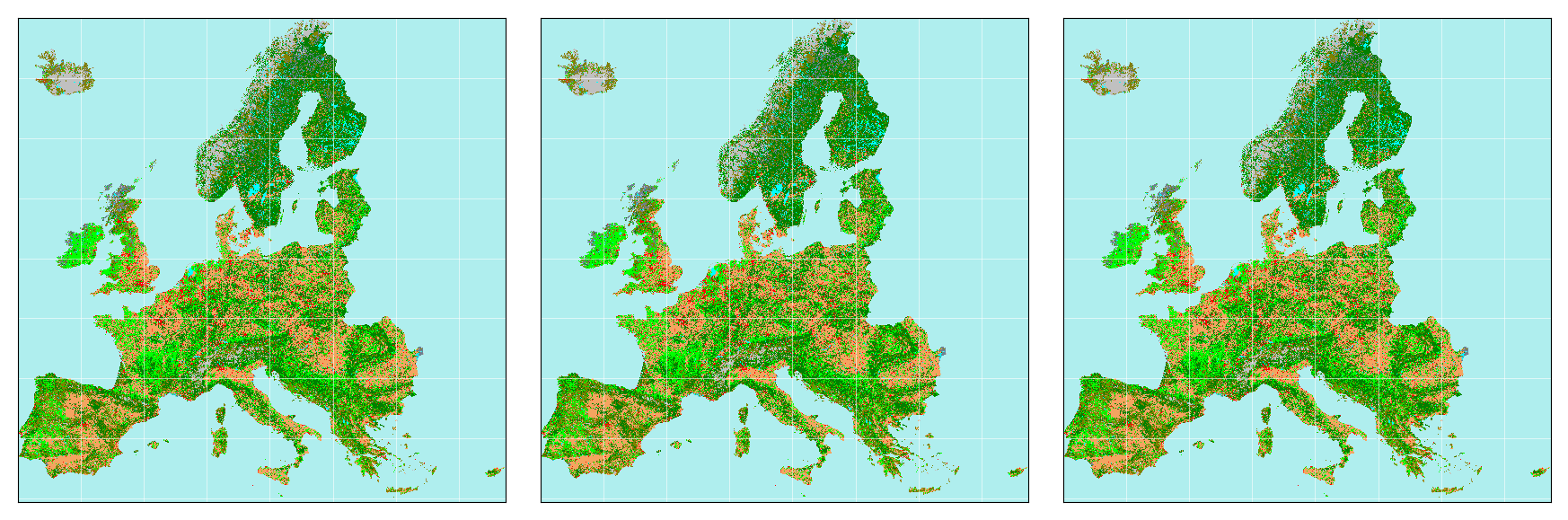
fig, ax = plt.subplots(facecolor='w', figsize=(7, 7))
ax.imshow(band_arr, cmap=cmap, norm=norm, interpolation='None', aspect='auto')
ax.grid(color='white', alpha=.7, linewidth=.6)
ax.set_xticklabels([])
ax.set_yticklabels([])
ax.tick_params(tick1On=False)
plt.savefig('test_clc.png', bbox_inches='tight', pad_inches=.2)
plt.close()
1
2
3
4
5
6
7
8
9
10
11
12
13
14
15
16
17
18
19
20
21
22
23
24
25
26
27
28
29
30
31
32
33
# Easy way to display a set of images horizontally/vertically

def vstack(images):
    if len(images) == 0:
        raise ValueError("Need 0 or more images")

    if isinstance(images[0], np.ndarray):
        images = [Image.fromarray(img) for img in images]
    width = max([img.size[0] for img in images])
    height = sum([img.size[1] for img in images])
    stacked = Image.new(images[0].mode, (width, height))

    y_pos = 0
    for img in images:
        stacked.paste(img, (0, y_pos))
        y_pos += img.size[1]
    return stacked

def hstack(images):
    if len(images) == 0:
        raise ValueError("Need 0 or more images")

    if isinstance(images[0], np.ndarray):
        images = [Image.fromarray(img) for img in images]
    width = sum([img.size[0] for img in images])
    height = max([img.size[1] for img in images])
    stacked = Image.new(images[0].mode, (width, height))

    x_pos = 0
    for img in images:
        stacked.paste(img, (x_pos, 0))
        x_pos += img.size[0]
    return stacked
1
2
3
4
img_set = []
for _ in range(3):
    img = cv2.cvtColor(cv2.imread('test_clc.png'), cv2.COLOR_BGR2RGB)
    img_set.append(img)
1
2
3
hstack(img_set)
# 단순 나열에 있어선, 만들어놓고 쓰기 편하긴 한데... annotate나 sub_title 같은 세부 작업이 어차피 필요함.
# 그냥 익숙한 multiple axes + for loop 쓰자...
Imperviousness density dataset
in the units of percent(%)
Needed directories:
- dataset/Imperviousness_1870_2020
1
2
3
4
5
6
impPath = os.path.join(BasePath, 'Imperviousness_1870_2020')
print(impPath)
print()

impContents = os.listdir(impPath)
print(impContents)
1
2
3
dataset/Imperviousness_1870_2020

['Imp_1870.tif', 'Imp_1880.tif', 'Imp_1890.tif', 'Imp_1900.tif', 'Imp_1910.tif', 'Imp_1920.tif', 'Imp_1930.tif', 'Imp_1940.tif', 'Imp_1950.tif', 'Imp_1955.tif', 'Imp_1960.tif', 'Imp_1965.tif', 'Imp_1970.tif', 'Imp_1975.tif', 'Imp_1980.tif', 'Imp_1985.tif', 'Imp_1990.tif', 'Imp_1995.tif', 'Imp_2000.tif', 'Imp_2001.tif', 'Imp_2002.tif', 'Imp_2003.tif', 'Imp_2004.tif', 'Imp_2005.tif', 'Imp_2006.tif', 'Imp_2007.tif', 'Imp_2008.tif', 'Imp_2009.tif', 'Imp_2010.tif', 'Imp_2011.tif', 'Imp_2012.tif', 'Imp_2013.tif', 'Imp_2014.tif', 'Imp_2015.tif', 'Imp_2016.tif', 'Imp_2017.tif', 'Imp_2018.tif', 'Imp_2019.tif', 'Imp_2020.tif']
1
2
3
4
5
# Open Imp_2020.tif
imp_sample = gdal.Open(os.path.join(impPath, impContents[-1]))

# Glimpse at Imp_2020.tif
AboutTif(imp_sample)
1
2
3
4
5
6
7
8
9
10
※ Number of bands: 1
--------------------
※ Raster size: 40300 rows x 38686 columns
-----------------------------------------
Raster description: dataset/Imperviousness_1870_2020/Imp_2020.tif
-----------------------------------------------------------------
++++++++++++++++++++++++++ For 1 band +++++++++++++++++++++++++++
Null value: 255.0
Mean: 0.518 / SD: 4.961 / min: 0.000 / max: 100.000
+++++++++++++++++++++++++++++++++++++++++++++++++++++++++++++++++
1
2
3
4
5
6
7
band_data = imp_sample.GetRasterBand(1)
band_arr = band_data.ReadAsArray()

# 0 % 인 지역이 굉장히 많다.
uni_val, counts = np.unique(band_arr.flatten(), return_counts=True)
uni_cnt_dict = dict(zip(uni_val, counts))
print(uni_cnt_dict)
1
{0: 1524045495, 1: 3172970, 2: 2526202, 3: 1937539, 4: 1614219, 5: 1390922, 6: 1215866, 7: 1070913, 8: 963898, 9: 867432, 10: 791911, 11: 728532, 12: 676894, 13: 626071, 14: 587461, 15: 553116, 16: 523460, 17: 493470, 18: 469269, 19: 446956, 20: 429956, 21: 407994, 22: 391830, 23: 377376, 24: 365155, 25: 350023, 26: 340728, 27: 329532, 28: 434482, 29: 376241, 30: 303639, 31: 297718, 32: 290710, 33: 283057, 34: 275980, 35: 271016, 36: 265487, 37: 258814, 38: 254430, 39: 248764, 40: 245665, 41: 238557, 42: 234874, 43: 231059, 44: 227653, 45: 283018, 46: 217780, 47: 213141, 48: 210700, 49: 204437, 50: 201606, 51: 197645, 52: 193288, 53: 188633, 54: 184766, 55: 180449, 56: 176575, 57: 171167, 58: 165792, 59: 161948, 60: 157694, 61: 151714, 62: 148491, 63: 142448, 64: 139310, 65: 133349, 66: 128242, 67: 123921, 68: 121416, 69: 115089, 70: 112060, 71: 108428, 72: 104475, 73: 100053, 74: 96511, 75: 93683, 76: 91675, 77: 87508, 78: 84339, 79: 81861, 80: 80284, 81: 76287, 82: 74117, 83: 71900, 84: 70784, 85: 67353, 86: 64721, 87: 62806, 88: 62024, 89: 58120, 90: 55768, 91: 54391, 92: 54442, 93: 50451, 94: 49498, 95: 48758, 96: 50573, 97: 46721, 98: 49979, 99: 60066, 100: 130209}
1
2
3
4
5
6
7
8
9
cList = ["dimgrey", "darkgrey", "sandybrown", "red"]
cmap = mpl.colors.LinearSegmentedColormap.from_list("", cList, len(cList))
cBounds = [1, 26, 51, 76, 101]
norm = mpl.colors.BoundaryNorm(cBounds, len(cList))
cmap.set_under('black')
cmap.set_over(color='white')

# .ipynb 에선 colorbar returned.
cmap
1
2
3
4
5
6
7
8
## 확인용 코드블럭: 특정 값에 내가 원하는 색상이 잘 적용되는지
test_value = 51
color = mpl.colors.rgb2hex(cmap(norm(test_value))[:3])

fig, ax = plt.subplots(facecolor='w', figsize=(3,3))
ax.scatter(.5, .5, s=5000, marker='s', transform=ax.transAxes, c=color)
ax.axis('off')
plt.show()

1
2
3
4
5
6
7
8
fig, ax = plt.subplots(facecolor='w', figsize=(8, 8))
ax.imshow(band_arr, cmap=cmap, norm=norm, interpolation='None', aspect='auto')

# ax.grid(color='white', alpha=.4, linewidth=.4)
ax.set_xticklabels([])
ax.set_yticklabels([])
ax.tick_params(tick1On=False)
plt.show()
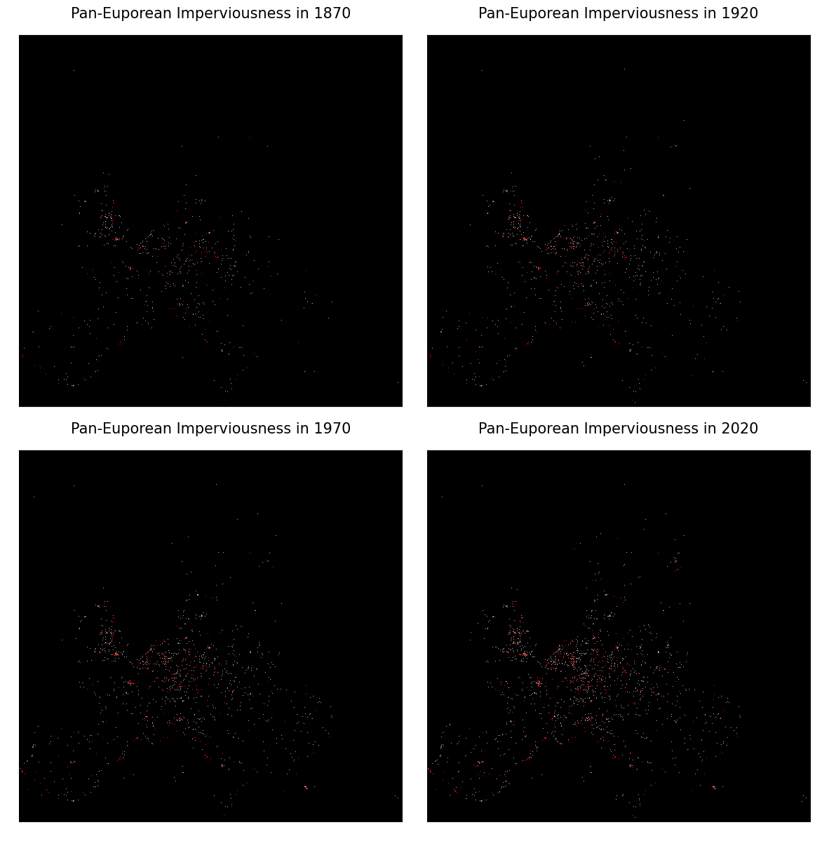
History of the imperviousness
Imp_1870 $ \Rightarrow $ Imp_1920 $ \Rightarrow $ Imp_1970 $ \Rightarrow $ Imp_2020
1
2
3
4
5
6
7
8
9
10
11
12
13
# 어느 정도 높은 부분만 보고 싶어서 아래와 같이 설정하였다.

# black < 1%
# 1% <= black < 34% : Normal imperviousness
# 34% <= darkgrey < 67% : Intermediate
# 67% <= red < 101% : High

cList = ["black", "darkgrey", "red"]
cmap = mpl.colors.LinearSegmentedColormap.from_list("", cList, len(cList))
cBounds = [1, 34, 67, 101]
norm = mpl.colors.BoundaryNorm(cBounds, len(cList))
cmap.set_under('black')
cmap.set_over(color='white')
1
2
3
4
5
6
7
8
9
10
11
12
13
14
15
16
17
18
19
20
years = [1870, 1920, 1970, 2020]
for yr in tqdm(years):
    target_path = os.path.join(impPath, f"Imp_{yr}.tif")
    print(target_path)
    one_imp = gdal.Open(target_path)

    # Get a raster image np.array
    band_data = one_imp.GetRasterBand(1)
    band_arr = band_data.ReadAsArray()

    # Save figures
    fig, ax = plt.subplots(facecolor='w', figsize=(8, 8))
    ax.imshow(band_arr, cmap=cmap, norm=norm, interpolation='None', aspect='auto')
    ax.set_xticklabels([])
    ax.set_yticklabels([])
    ax.tick_params(tick1On=False)

    save_name = f"ImpMap_{yr}.png"
    plt.savefig(save_name, dpi=200, bbox_inches='tight', pad_inches=.2)
    plt.close()
1
2
3
4
5
6
7
8
9
10
11
12
13
14
15
16
17
18
19
20
21
  0%|          | 0/4 [00:00<?, ?it/s]

dataset/Imperviousness_1870_2020/Imp_1870.tif


 25%|██▌       | 1/4 [00:32<01:36, 32.19s/it]

dataset/Imperviousness_1870_2020/Imp_1920.tif


 50%|█████     | 2/4 [01:03<01:03, 31.89s/it]

dataset/Imperviousness_1870_2020/Imp_1970.tif


 75%|███████▌  | 3/4 [01:35<00:31, 31.80s/it]

dataset/Imperviousness_1870_2020/Imp_2020.tif


100%|██████████| 4/4 [02:07<00:00, 31.82s/it]
1
2
3
4
5
6
7
8
9
10
11
12
13
14
# Plotting the history of Imperviousness
fig, axe = plt.subplots(nrows=2, ncols=2, facecolor='w', figsize=(15, 15))
for ax, yr in zip(axe.flatten(), years):
    filename = f"ImpMap_{yr}.png"
    img = mpl.image.imread(filename)

    ax.imshow(img, interpolation='None', aspect='auto')
    ax.axis('off')

    title = f"Pan-Euporean Imperviousness in {yr}"
    ax.set_title(title, fontsize=15)

plt.subplots_adjust(wspace=.001, hspace=.05)
plt.show()
GDP / Fixed Assets / Population dataset
나머지 세 변수에 대한 데이터셋도 한 번에 살펴보자.
Needed directories:
- GDP: dataset/GDP_1870_2020
- Fixed Asssets: dataset/Fixed_asset_value_1870_2020
- Population: dataset/Population_1870_2020
1
2
3
4
5
6
7
8
9
10
tif_list = []
for folder in ['GDP_1870_2020', 'Fixed_asset_value_1870_2020', 'Population_1870_2020']:
    folder_path = os.path.join(BasePath, folder)
    tif_name = os.listdir(folder_path)[-1] # 샘플로 2020년 데이터만 확인
    msg = f"< {tif_name} >"
    print(f"{msg:=^100}")
    tf = gdal.Open(os.path.join(folder_path, tif_name))
    AboutTif(tf)
    tif_list.append(tf)
    print()
1
2
3
4
5
6
7
8
9
10
11
12
13
14
15
16
17
18
19
20
21
22
23
24
25
26
27
28
29
30
31
32
33
34
35
=======================================< GDP_100m_2020.tif >========================================
※ Number of bands: 1
--------------------
※ Raster size: 40300 rows x 38686 columns
-----------------------------------------
Raster description: dataset/GDP_1870_2020/GDP_100m_2020.tif
-----------------------------------------------------------
+++++++++++++++++++++++ For 1 band ++++++++++++++++++++++++
Null value: 65535.0
Mean: 10783.017 / SD: 198597.734 / min: 0.000 / max: 316835788.000
+++++++++++++++++++++++++++++++++++++++++++++++++++++++++++

========================================< FA_100m_2020.tif >========================================
※ Number of bands: 1
--------------------
※ Raster size: 40300 rows x 38686 columns
-----------------------------------------
Raster description: dataset/Fixed_asset_value_1870_2020/FA_100m_2020.tif
------------------------------------------------------------------------
++++++++++++++++++++++++++++++ For 1 band ++++++++++++++++++++++++++++++
Null value: 65535.0
Mean: 61861.556 / SD: 1083751.583 / min: 0.000 / max: 1304974474.000
++++++++++++++++++++++++++++++++++++++++++++++++++++++++++++++++++++++++

====================================< Population_100m_2020.tif >====================================
※ Number of bands: 1
--------------------
※ Raster size: 40300 rows x 38686 columns
-----------------------------------------
Raster description: dataset/Population_1870_2020/Population_100m_2020.tif
-------------------------------------------------------------------------
++++++++++++++++++++++++++++++ For 1 band +++++++++++++++++++++++++++++++
Null value: 65535.0
Mean: 0.346 / SD: 5.617 / min: 0.000 / max: 6101.000
+++++++++++++++++++++++++++++++++++++++++++++++++++++++++++++++++++++++++
나머지 데이터셋들도 역시 40,300 by 38,686 크기의 raster 데이터임을 확인할 수 있다.
각 데이터셋들의 colormap bound 는 data unique values들의 25th, 50th, 75th, 100th percentile 지점들로 나누고 색을 할당하자.
1
2
3
4
# GDP_100m_2020.tif
tf_one_test = tif_list[0]
test_band = tf_one_test.GetRasterBand(1)
test_val = test_band.ReadAsArray().flatten()
1
2
3
%%timeit -o
test_uni = pd.unique(test_val)
np.sort(test_uni)
1
2
3
6.67 s ± 18.3 ms per loop (mean ± std. dev. of 7 runs, 1 loop each)

<TimeitResult : 6.67 s ± 18.3 ms per loop (mean ± std. dev. of 7 runs, 1 loop each)>
1
2
%%timeit -o
np.unique(test_val)
1
2
3
1min 37s ± 48.6 ms per loop (mean ± std. dev. of 7 runs, 1 loop each)

<TimeitResult : 1min 37s ± 48.6 ms per loop (mean ± std. dev. of 7 runs, 1 loop each)>
np.unique()는 “unique 추출 + sort” 두 작업을 한번에 수행해서 느리다지만, 위 결과에선 pandas unique(without sorting) + numpy sort 로 개별수행해도 np.unique()가 (좀 심하게)훨씬 느리다는 것을 확인할 수 있다. 그러니까..
왠만하면 np.unique는 쓰지 말자…
다만, np.unique()의 return_counts 옵션(unique 추출 + 각 요소들의 포함 갯수 산출)은 꽤 요긴하다.
1
2
3
4
5
6
7
8
9
10
11
12
13
14
15
16
17
18
19
20
21
cList = ["dimgrey", "darkgrey", "sandybrown", "red"]
cmap = mpl.colors.LinearSegmentedColormap.from_list("", cList, len(cList))
cmap.set_under(color='black')
cmap.set_over(color='red')

norm_list = [] # a list of norms
for i in tqdm(range(len(tif_list))):
    if i == 0:
        img_cube = np.zeros((40300, 38686, 3)) # 여기다 차곡차곡 담을거임

    tf_band = tif_list[i].GetRasterBand(1)
    tf_img = tf_band.ReadAsArray()
    img_cube[:, :, i] = tf_img

    # 0 값은 다른 특정 색으로 할당할 것이기 때문에 2-th smallest 값을 minimum bound로 사용한다.
    tf_val = np.sort(pd.unique(tf_img.flatten()))
    second_min_val = [tf_val[1]]
    cBounds = np.percentile(tf_val, q=[25, 50, 75, 100])
    cBounds = second_min_val + cBounds
    norm = mpl.colors.BoundaryNorm(cBounds, len(cList))
    norm_list.append(norm)
1
100%|██████████| 3/3 [01:19<00:00, 26.51s/it]
1
2
3
4
5
6
7
fig, axe = plt.subplots(nrows=1, ncols=3, facecolor='w', figsize=(32, 10))
for ii, ax in enumerate(axe.flatten()):
    ax.imshow(img_cube[:, :, ii], cmap=cmap, norm=norm_list[ii], interpolation='None', aspect='auto')
    ax.axis('off')

plt.subplots_adjust(wspace=.01)
plt.show()
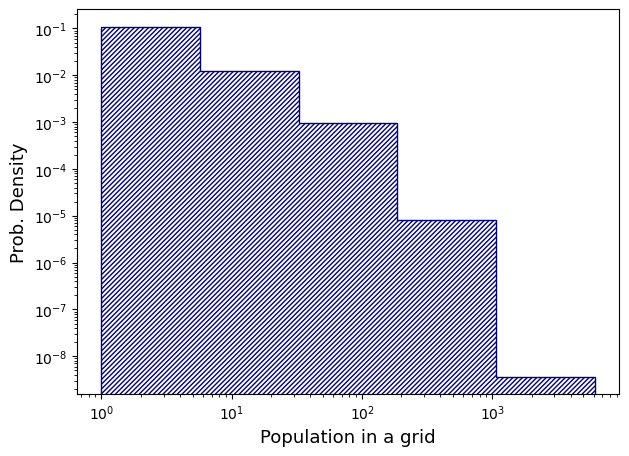
Population tif 도 마찬가지로 unique value 들의 percentile binning 을 했는데, 시각화 표현이 잘 안된다.
작은 value 값을 갖는 grid들이 압도적으로 많아서일까? 한번 들여다보자.
1
2
3
4
5
6
# Population_100m_2020.tif

pop_sample = tif_list[-1]
pop_band = pop_sample.GetRasterBand(1)
pop_img = pop_band.ReadAsArray()
pop_value = pop_img.flatten()
1
2
3
uni_val, counts = np.unique(pop_value, return_counts=True)
uni_cnt_dict = dict(zip(uni_val, counts))
print(uni_cnt_dict)
1
{0: 1528788255, 1: 5616910, 2: 4625796, 3: 2361889, 4: 1692013, 5: 1293178, 6: 1030204, 7: 864348, 8: 743619, 9: 646465, 10: 571085, 11: 523865, 12: 477831, 13: 434368, 14: 398074, 15: 364568, 16: 342373, 17: 314458, 18: 298100, 19: 284539, 20: 261122, 21: 250953, 22: 237309, 23: 226742, 24: 213230, 25: 205022, 26: 197579, 27: 187457, 28: 177734, 29: 167426, 30: 165235, 31: 156526, 32: 151312, 33: 144000, 34: 142406, 35: 132978, 36: 130958, 37: 125624, 38: 123557, 39: 118337, 40: 111036, 41: 105577, 42: 107688, 43: 101496, 44: 97614, 45: 94516, 46: 90571, 47: 88663, 48: 84931, 49: 83687, 50: 81981, 51: 78055, 52: 74375, 53: 72901, 54: 71550, 55: 68651, 56: 66477, 57: 65514, 58: 62739, 59: 61359, 60: 59226, 61: 58845, 62: 55996, 63: 52752, 64: 53388, 65: 50568, 66: 47667, 67: 47225, 68: 45564, 69: 44776, 70: 44618, 71: 42591, 72: 40919, 73: 38221, 74: 38040, 75: 36482, 76: 35244, 77: 34152, 78: 33067, 79: 31861, 80: 31315, 81: 30201, 82: 29244, 83: 29307, 84: 27696, 85: 26858, 86: 25243, 87: 25164, 88: 23864, 89: 23460, 90: 22638, 91: 21767, 92: 21208, 93: 20774, 94: 19822, 95: 19220, 96: 18885, 97: 18155, 98: 17684, 99: 17437, 100: 16645, 101: 15765, 102: 15454, 103: 15290, 104: 14596, 105: 14251, 106: 13668, 107: 14078, 108: 13662, 109: 12880, 110: 12574, 111: 12782, 112: 11738, 113: 11619, 114: 11243, 115: 11171, 116: 10902, 117: 10408, 118: 10386, 119: 9887, 120: 9664, 121: 9678, 122: 9046, 123: 8933, 124: 8879, 125: 8685, 126: 8378, 127: 8332, 128: 8034, 129: 7643, 130: 7719, 131: 7500, 132: 7476, 133: 7064, 134: 7255, 135: 7094, 136: 6874, 137: 6308, 138: 6300, 139: 6134, 140: 6177, 141: 5656, 142: 6014, 143: 5807, 144: 5646, 145: 5446, 146: 5754, 147: 5349, 148: 5107, 149: 5049, 150: 4903, 151: 4852, 152: 4929, 153: 4817, 154: 4210, 155: 4554, 156: 4208, 157: 4276, 158: 4371, 159: 4371, 160: 4122, 161: 4047, 162: 4103, 163: 3838, 164: 3667, 165: 3765, 166: 3571, 167: 3514, 168: 3544, 169: 3676, 170: 3438, 171: 3396, 172: 3473, 173: 3302, 174: 3296, 175: 3166, 176: 3137, 177: 3057, 178: 3219, 179: 3010, 180: 2855, 181: 2803, 182: 2897, 183: 2894, 184: 2729, 185: 2702, 186: 2564, 187: 2802, 188: 2631, 189: 2480, 190: 2481, 191: 2307, 192: 2363, 193: 2601, 194: 2340, 195: 2298, 196: 2247, 197: 2301, 198: 2201, 199: 2194, 200: 2123, 201: 2210, 202: 2113, 203: 2067, 204: 1991, 205: 2125, 206: 1868, 207: 1914, 208: 2064, 209: 1958, 210: 2069, 211: 1956, 212: 1925, 213: 1681, 214: 1903, 215: 1637, 216: 1668, 217: 1567, 218: 1654, 219: 1757, 220: 1594, 221: 1648, 222: 1607, 223: 1692, 224: 1391, 225: 1572, 226: 1453, 227: 1534, 228: 1530, 229: 1462, 230: 1444, 231: 1389, 232: 1328, 233: 1466, 234: 1271, 235: 1418, 236: 1394, 237: 1272, 238: 1346, 239: 1241, 240: 1276, 241: 1300, 242: 1197, 243: 1220, 244: 1241, 245: 1195, 246: 1235, 247: 1219, 248: 1170, 249: 1103, 250: 1172, 251: 1084, 252: 1107, 253: 1160, 254: 999, 255: 993, 256: 1047, 257: 1052, 258: 1027, 259: 1033, 260: 1003, 261: 940, 262: 954, 263: 937, 264: 913, 265: 1015, 266: 938, 267: 922, 268: 921, 269: 875, 270: 825, 271: 883, 272: 784, 273: 881, 274: 916, 275: 835, 276: 843, 277: 887, 278: 691, 279: 707, 280: 759, 281: 791, 282: 809, 283: 801, 284: 754, 285: 721, 286: 684, 287: 784, 288: 719, 289: 744, 290: 661, 291: 718, 292: 692, 293: 668, 294: 712, 295: 745, 296: 645, 297: 650, 298: 633, 299: 647, 300: 658, 301: 642, 302: 601, 303: 596, 304: 540, 305: 611, 306: 669, 307: 601, 308: 581, 309: 521, 310: 558, 311: 479, 312: 561, 313: 547, 314: 566, 315: 554, 316: 545, 317: 530, 318: 533, 319: 567, 320: 460, 321: 501, 322: 468, 323: 494, 324: 554, 325: 513, 326: 494, 327: 441, 328: 533, 329: 380, 330: 468, 331: 423, 332: 437, 333: 424, 334: 536, 335: 466, 336: 361, 337: 416, 338: 426, 339: 354, 340: 411, 341: 433, 342: 419, 343: 398, 344: 384, 345: 424, 346: 353, 347: 417, 348: 407, 349: 303, 350: 395, 351: 349, 352: 368, 353: 448, 354: 329, 355: 344, 356: 345, 357: 321, 358: 377, 359: 343, 360: 356, 361: 314, 362: 362, 363: 353, 364: 312, 365: 309, 366: 294, 367: 338, 368: 307, 369: 329, 370: 306, 371: 286, 372: 290, 373: 279, 374: 260, 375: 319, 376: 312, 377: 326, 378: 289, 379: 279, 380: 291, 381: 300, 382: 270, 383: 276, 384: 270, 385: 284, 386: 271, 387: 268, 388: 282, 389: 312, 390: 230, 391: 263, 392: 238, 393: 276, 394: 239, 395: 281, 396: 225, 397: 232, 398: 257, 399: 207, 400: 239, 401: 238, 402: 204, 403: 241, 404: 214, 405: 193, 406: 155, 407: 232, 408: 244, 409: 186, 410: 220, 411: 208, 412: 267, 413: 197, 414: 266, 415: 197, 416: 162, 417: 204, 418: 176, 419: 212, 420: 191, 421: 188, 422: 180, 423: 164, 424: 152, 425: 225, 426: 179, 427: 184, 428: 173, 429: 201, 430: 135, 431: 211, 432: 178, 433: 190, 434: 202, 435: 144, 436: 167, 437: 159, 438: 169, 439: 144, 440: 138, 441: 158, 442: 158, 443: 157, 444: 224, 445: 167, 446: 154, 447: 144, 448: 214, 449: 126, 450: 126, 451: 126, 452: 124, 453: 192, 454: 139, 455: 127, 456: 162, 457: 147, 458: 147, 459: 134, 460: 137, 461: 108, 462: 115, 463: 110, 464: 131, 465: 125, 466: 122, 467: 143, 468: 139, 469: 135, 470: 137, 471: 94, 472: 117, 473: 119, 474: 102, 475: 126, 476: 80, 477: 189, 478: 104, 479: 107, 480: 98, 481: 92, 482: 131, 483: 118, 484: 97, 485: 99, 486: 92, 487: 119, 488: 101, 489: 83, 490: 94, 491: 87, 492: 92, 493: 94, 494: 103, 495: 75, 496: 111, 497: 82, 498: 105, 499: 74, 500: 69, 501: 83, 502: 73, 503: 81, 504: 93, 505: 179, 506: 83, 507: 98, 508: 74, 509: 83, 510: 64, 511: 81, 512: 90, 513: 72, 514: 76, 515: 80, 516: 106, 517: 71, 518: 86, 519: 74, 520: 87, 521: 81, 522: 74, 523: 65, 524: 97, 525: 80, 526: 80, 527: 74, 528: 77, 529: 78, 530: 67, 531: 72, 532: 88, 533: 69, 534: 94, 535: 46, 536: 81, 537: 60, 538: 101, 539: 72, 540: 60, 541: 72, 542: 84, 543: 51, 544: 56, 545: 44, 546: 69, 547: 64, 548: 90, 549: 74, 550: 44, 551: 58, 552: 62, 553: 66, 554: 56, 555: 65, 556: 65, 557: 51, 558: 52, 559: 66, 560: 75, 561: 84, 562: 39, 563: 83, 564: 44, 565: 44, 566: 60, 567: 54, 568: 55, 569: 46, 570: 50, 571: 72, 572: 46, 573: 58, 574: 54, 575: 63, 576: 58, 577: 51, 578: 44, 579: 56, 580: 41, 581: 41, 582: 55, 583: 41, 584: 38, 585: 53, 586: 56, 587: 50, 588: 34, 589: 53, 590: 26, 591: 41, 592: 34, 593: 39, 594: 48, 595: 51, 596: 39, 597: 34, 598: 40, 599: 36, 600: 40, 601: 30, 602: 27, 603: 30, 604: 43, 605: 39, 606: 62, 607: 39, 608: 44, 609: 77, 610: 51, 611: 43, 612: 36, 613: 33, 614: 25, 615: 27, 616: 40, 617: 35, 618: 34, 619: 30, 620: 52, 621: 45, 622: 18, 623: 31, 624: 40, 625: 32, 626: 27, 627: 35, 628: 32, 629: 31, 630: 31, 631: 22, 632: 34, 633: 38, 634: 39, 635: 21, 636: 25, 637: 28, 638: 25, 639: 31, 640: 33, 641: 28, 642: 25, 643: 20, 644: 40, 645: 28, 646: 30, 647: 31, 648: 34, 649: 35, 650: 36, 651: 13, 652: 23, 653: 29, 654: 25, 655: 32, 656: 23, 657: 64, 658: 20, 659: 27, 660: 21, 661: 18, 662: 26, 663: 31, 664: 19, 665: 24, 666: 20, 667: 29, 668: 12, 669: 22, 670: 26, 671: 18, 672: 22, 673: 24, 674: 27, 675: 44, 676: 14, 677: 38, 678: 10, 679: 12, 680: 24, 681: 46, 682: 28, 683: 25, 684: 8, 685: 18, 686: 11, 687: 24, 688: 15, 689: 23, 690: 23, 691: 13, 692: 18, 693: 16, 694: 24, 695: 18, 696: 17, 697: 29, 698: 12, 699: 19, 700: 23, 701: 11, 702: 13, 703: 20, 704: 34, 705: 14, 706: 19, 707: 10, 708: 27, 709: 23, 710: 13, 711: 9, 712: 16, 713: 17, 714: 12, 715: 10, 716: 13, 717: 20, 718: 17, 719: 10, 720: 22, 721: 14, 722: 6, 723: 20, 724: 10, 725: 12, 726: 25, 727: 9, 728: 8, 729: 16, 730: 15, 731: 19, 732: 16, 733: 7, 734: 5, 735: 13, 736: 13, 737: 3, 738: 10, 739: 12, 740: 8, 741: 28, 742: 13, 743: 11, 744: 25, 745: 9, 746: 10, 747: 12, 748: 15, 749: 16, 750: 12, 751: 10, 752: 5, 753: 6, 754: 9, 755: 13, 756: 18, 757: 9, 758: 10, 759: 15, 760: 7, 761: 10, 762: 11, 763: 4, 764: 25, 765: 8, 766: 30, 767: 12, 768: 7, 769: 14, 770: 16, 771: 9, 772: 11, 773: 7, 774: 31, 775: 3, 776: 12, 777: 2, 778: 13, 779: 19, 780: 14, 781: 6, 782: 5, 783: 13, 784: 5, 785: 6, 786: 8, 787: 8, 788: 11, 789: 4, 790: 9, 791: 10, 792: 9, 793: 13, 794: 8, 795: 15, 796: 3, 797: 6, 798: 11, 799: 9, 800: 5, 801: 9, 802: 10, 803: 8, 804: 5, 805: 30, 806: 7, 807: 6, 808: 5, 809: 4, 810: 4, 811: 5, 812: 24, 813: 2, 814: 8, 815: 4, 816: 9, 817: 6, 818: 15, 819: 12, 820: 6, 821: 8, 822: 5, 823: 9, 824: 4, 825: 6, 826: 5, 827: 7, 828: 3, 829: 3, 830: 7, 831: 3, 832: 11, 833: 11, 834: 4, 835: 3, 836: 4, 837: 18, 838: 6, 839: 2, 840: 2, 841: 5, 842: 9, 843: 14, 844: 5, 845: 7, 846: 2, 847: 10, 848: 7, 849: 4, 850: 4, 851: 28, 852: 7, 853: 4, 854: 15, 855: 7, 856: 3, 857: 4, 858: 3, 860: 7, 862: 5, 863: 13, 864: 5, 865: 3, 866: 1, 867: 2, 868: 5, 869: 4, 870: 6, 871: 7, 872: 5, 873: 7, 874: 7, 875: 2, 876: 6, 877: 3, 878: 56, 879: 5, 880: 3, 881: 5, 882: 2, 883: 4, 884: 2, 885: 3, 886: 5, 887: 2, 888: 2, 889: 3, 890: 4, 891: 1, 892: 3, 893: 3, 894: 3, 895: 5, 896: 7, 897: 2, 898: 4, 899: 4, 901: 8, 902: 3, 903: 14, 904: 3, 905: 5, 906: 4, 907: 1, 908: 2, 909: 4, 910: 4, 911: 3, 912: 1, 913: 1, 914: 1, 915: 2, 916: 3, 917: 3, 918: 3, 919: 3, 920: 1, 921: 3, 922: 2, 924: 2, 925: 6, 927: 3, 928: 4, 929: 4, 930: 4, 931: 1, 932: 3, 933: 6, 934: 2, 936: 2, 937: 4, 938: 1, 940: 7, 942: 1, 943: 1, 945: 2, 946: 4, 947: 1, 948: 1, 949: 2, 950: 7, 951: 2, 952: 4, 953: 2, 954: 4, 955: 4, 956: 1, 957: 1, 959: 3, 960: 1, 961: 7, 962: 1, 963: 5, 965: 4, 966: 1, 967: 4, 968: 3, 969: 2, 970: 1, 971: 2, 972: 1, 974: 2, 975: 2, 976: 5, 977: 1, 978: 4, 979: 1, 981: 1, 982: 1, 983: 1, 984: 3, 985: 5, 986: 1, 987: 2, 988: 3, 990: 1, 991: 14, 993: 3, 994: 6, 995: 1, 997: 6, 998: 4, 999: 5, 1000: 9, 1001: 2, 1004: 8, 1005: 3, 1006: 3, 1007: 1, 1008: 4, 1009: 2, 1010: 2, 1011: 2, 1012: 4, 1013: 1, 1014: 4, 1015: 1, 1016: 1, 1018: 1, 1019: 2, 1020: 7, 1021: 1, 1023: 1, 1024: 1, 1025: 1, 1026: 1, 1027: 2, 1030: 1, 1032: 2, 1033: 2, 1034: 1, 1035: 3, 1036: 1, 1037: 1, 1038: 6, 1039: 3, 1042: 2, 1043: 1, 1044: 2, 1045: 3, 1046: 10, 1047: 2, 1048: 4, 1049: 2, 1050: 1, 1051: 5, 1052: 2, 1054: 1, 1055: 1, 1061: 1, 1064: 2, 1065: 3, 1066: 3, 1068: 1, 1069: 1, 1070: 5, 1071: 1, 1072: 7, 1075: 1, 1076: 2, 1077: 1, 1078: 4, 1079: 3, 1080: 1, 1084: 2, 1085: 2, 1086: 3, 1087: 1, 1088: 1, 1089: 1, 1091: 1, 1092: 4, 1093: 3, 1095: 3, 1097: 6, 1100: 1, 1101: 1, 1102: 3, 1103: 1, 1104: 3, 1106: 1, 1108: 2, 1109: 1, 1112: 1, 1114: 2, 1115: 1, 1117: 1, 1124: 2, 1126: 2, 1127: 3, 1130: 3, 1132: 2, 1133: 2, 1134: 1, 1136: 1, 1137: 1, 1139: 1, 1142: 3, 1143: 1, 1146: 1, 1148: 2, 1150: 1, 1152: 1, 1155: 1, 1158: 1, 1160: 1, 1161: 2, 1164: 2, 1165: 2, 1167: 1, 1170: 1, 1172: 1, 1175: 3, 1176: 1, 1178: 1, 1181: 1, 1184: 2, 1185: 2, 1191: 4, 1193: 1, 1194: 1, 1195: 1, 1196: 1, 1198: 1, 1200: 2, 1201: 1, 1204: 1, 1207: 1, 1209: 2, 1211: 1, 1216: 1, 1220: 3, 1223: 1, 1225: 3, 1226: 1, 1230: 9, 1232: 1, 1234: 1, 1237: 2, 1239: 1, 1247: 2, 1249: 1, 1252: 3, 1256: 17, 1260: 2, 1262: 1, 1263: 10, 1264: 2, 1266: 1, 1267: 1, 1269: 2, 1272: 1, 1274: 1, 1275: 1, 1278: 1, 1279: 1, 1281: 2, 1285: 1, 1290: 1, 1291: 1, 1298: 2, 1304: 1, 1306: 2, 1309: 3, 1316: 2, 1318: 1, 1321: 1, 1332: 2, 1336: 1, 1341: 1, 1346: 1, 1352: 1, 1353: 3, 1355: 1, 1358: 1, 1359: 2, 1360: 1, 1372: 1, 1373: 1, 1374: 1, 1380: 1, 1400: 9, 1402: 1, 1405: 2, 1409: 3, 1424: 1, 1428: 2, 1432: 1, 1437: 1, 1440: 1, 1442: 1, 1451: 1, 1452: 2, 1455: 1, 1459: 1, 1475: 2, 1484: 1, 1488: 1, 1493: 1, 1494: 1, 1495: 1, 1503: 1, 1510: 1, 1514: 1, 1516: 1, 1530: 1, 1550: 1, 1571: 1, 1572: 1, 1577: 1, 1581: 1, 1585: 1, 1594: 8, 1599: 1, 1615: 1, 1617: 1, 1620: 1, 1627: 1, 1628: 1, 1631: 1, 1652: 2, 1658: 1, 1664: 1, 1671: 1, 1678: 1, 1679: 1, 1681: 1, 1688: 2, 1698: 1, 1704: 1, 1712: 1, 1714: 1, 1724: 4, 1727: 2, 1730: 2, 1739: 1, 1740: 1, 1748: 1, 1767: 1, 1770: 1, 1780: 1, 1781: 1, 1788: 1, 1824: 1, 1838: 1, 1851: 1, 1854: 1, 1863: 1, 1864: 1, 1871: 1, 1885: 1, 1901: 1, 1917: 1, 1919: 1, 1924: 1, 1930: 1, 1966: 1, 1967: 2, 1968: 2, 1979: 1, 1986: 3, 1988: 1, 1998: 2, 2004: 1, 2023: 1, 2025: 4, 2038: 1, 2041: 1, 2053: 1, 2064: 1, 2083: 1, 2088: 1, 2089: 1, 2102: 3, 2114: 1, 2155: 1, 2168: 1, 2183: 1, 2197: 1, 2211: 1, 2225: 1, 2226: 2, 2232: 1, 2242: 1, 2254: 1, 2273: 1, 2287: 2, 2290: 1, 2307: 1, 2323: 1, 2341: 1, 2350: 1, 2360: 1, 2361: 2, 2380: 1, 2385: 1, 2387: 1, 2430: 1, 2442: 1, 2461: 2, 2469: 1, 2479: 1, 2486: 1, 2499: 3, 2519: 2, 2530: 1, 2551: 2, 2554: 2, 2556: 1, 2562: 1, 2573: 2, 2579: 1, 2580: 1, 2595: 5, 2607: 2, 2618: 3, 2630: 1, 2637: 1, 2642: 1, 2654: 1, 2667: 2, 2679: 1, 2690: 1, 2691: 1, 2702: 2, 2704: 4, 2717: 2, 2726: 1, 2730: 2, 2738: 1, 2751: 1, 2763: 2, 2771: 4, 2785: 1, 2789: 1, 2799: 2, 2801: 3, 2809: 1, 2813: 1, 2814: 1, 2825: 2, 2828: 1, 2836: 7, 2840: 1, 2842: 1, 2843: 4, 2867: 2, 2874: 1, 2905: 1, 2908: 1, 2922: 4, 2950: 1, 2955: 1, 2973: 1, 2990: 2, 2994: 2, 3001: 1, 3008: 1, 3024: 1, 3039: 2, 3043: 1, 3061: 1, 3084: 3, 3146: 1, 3190: 3, 3205: 1, 3219: 5, 3310: 5, 3390: 1, 3448: 4, 3484: 1, 3614: 5, 3773: 1, 3818: 3, 3915: 1, 4024: 1, 4085: 3, 4149: 1, 4379: 8, 4711: 1, 6101: 1}
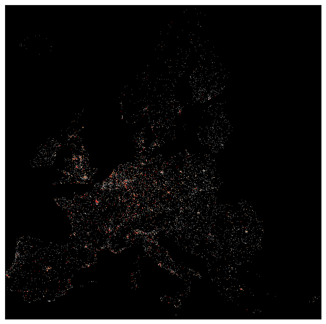
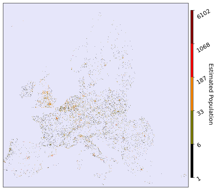
예상대로, 40300 x 38686 개의 그리드 규모(약 15억 5천만)에 15억 2천만개 그리드 정도가 population 0으로 확인된다. 그리고 value가 높을 수록 해당하는 그리드 갯수는 exponential보다 더욱 가파르게 감소한다. 그래서 약간의 대안으로 Population 데이터 시각화는 logbinning(값이 커질수록 더욱 큰 data range)으로 colorbar bound 들을 잡기로 했다.
1
2
3
4
5
6
7
8
9
10
11
fig, ax = plt.subplots(facecolor='w', figsize=(7, 5))

logbins = np.logspace(np.log10(1), np.log10(pop_value.max()), 6)
ax.hist(pop_value, bins=logbins, density=True, color='navy', histtype='step', hatch='///////')

ax.set_ylabel("Prob. Density", fontsize=13)
ax.set_xlabel("Population in a grid", fontsize=13)
ax.set_xscale('log')
ax.set_yscale('log')

plt.show()
1
2
3
4
5
6
7
cList = ["black", "olive", "darkorange", "red", "darkred"]
cmap = mpl.colors.LinearSegmentedColormap.from_list("", cList, len(cList))
cBounds = np.logspace(np.log10(1), np.log10(pop_value.max()+1), 6)
norm = mpl.colors.BoundaryNorm(cBounds, len(cList))
cmap.set_under('lavender')
cmap.set_over(color='white')
cmap
1
2
3
4
5
6
7
8
9
10
11
12
13
fig, ax = plt.subplots(facecolor='w', figsize=(8, 8))
im = ax.imshow(pop_img, cmap=cmap, norm=norm, interpolation='None', aspect='auto')

ax.set_xticklabels([])
ax.set_yticklabels([])
ax.tick_params(tick1On=False)

cbar_ax = fig.add_axes([0.91, 0.15, 0.01, 0.7])
cbar = fig.colorbar(im, cax=cbar_ax)
cbar.set_label(label="Estimated Population", size=14, rotation=270)
cbar.ax.tick_params(labelsize=14, rotation=30)

plt.show()
fin