

들어가며
‘핀란드의 수도, 헬싱키의 통행시간 데이터’를 살펴본 내용이다. 데이터 전처리 및 상세 내용은 아래 논문을 참조하면 된다.
< Longitudinal spatial dataset on travel times and distances by different travel modes in Helsinki Region. > - Tenkanen, Henrikki, and Tuuli Toivonen., Scientific Data (Mar, 2020)
본 논문의 핀란드 연구팀은 추후 [(2022, Scientific Data) Bergroth, Claudia, et al.]로 ‘헬싱키 생활인구 데이터’를 발표하게 된다.
Travel Time in Helsinki, Finland
1
2
3
4
5
6
7
8
9
10
11
12
13
import os
import json
import numpy as np
import pandas as pd
import geopandas as gpd
import matplotlib.pyplot as plt
import matplotlib as mpl
import networkx as nx
import contextily as cx
import folium
from tqdm import tqdm
from folium.elements import Figure
from collections import defaultdict
Data Acquisition
- 본 연구팀은 해당 데이터셋을 총 3개연도 데이터셋(2013년, 2015년, 2018년)으로 나누어 배포하고 있다.
- 터미널에서 wget URL을 통해 데이터셋을 내려받을 수 있다. (아래 Command line 참고)
1
2
3
4
>>> wget https://zenodo.org/record/3247564/files/HelsinkiRegion_TravelTimeMatrix2013.zip?download=1  # 2013년 데이터 (2.3 GB)
>>> wget https://zenodo.org/record/3247564/files/HelsinkiRegion_TravelTimeMatrix2015.zip?download=1  # 2015년 데이터 (3.7 GB)
>>> wget https://zenodo.org/record/3247564/files/HelsinkiRegion_TravelTimeMatrix2018.zip?download=1  # 2018년 데이터 (4.4 GB)
>>> wget https://zenodo.org/record/3247564/files/MetropAccess_YKR_grid.zip?download=1 # YKR Grid shapefiles
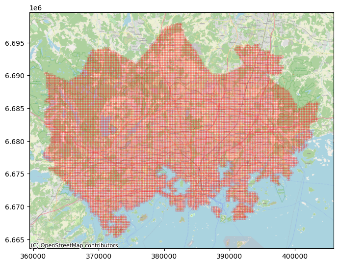
- YKR Grid는 핀란드 정부기관이 통계 조사를 위해 250m by 250m 크기의 셀로 핀란드를 나눈 지질학적 격자다. (그래서 본 연구팀에선 statistical grid라고도 한다.)
- 핀란드의 수도, 헬싱키를 포괄하는 YKR Grid는 총 13,231개이다.
- 각각의 YKR Grid는 YKR_ID로 구분된다.
- 연도별 데이터셋을 들여다 보면 아래와 같은 동일한 구조로 나눠져 있다.
1
2
3
4
5
6
7
8
9
10
11
2018/                   # 2018년 데이터 (4.4 GB)
├── 5785xxx
│   ├── travel_times_to_\ 5785640.txt (Ex-1)
│   ├── travel_times_to_\ 5785641.txt
│   ├── travel_times_to_\ 5785642.txt
│   └── travel_times_to_\ 5785643.txt
├── 5787xxx
├── ...
├── 6016xxx
├── 6018xxx
└── METADATA_Helsinki-Region-Travel-Time-Matrix-2018.txt
- 하나의 특정 YKR Grid을 대상으로 하는 개별 데이터들로 나눠져 있다.
- Ex-1 데이터를 예시로 들면, 총 13,231개의 YKR Grid들이 5785640 이라는 YKR_ID를 갖는 Grid로 향할 경우의 통행 시간들이 기록되어 있다.
- 각 sub-directory 안에 있는 .txt 파일들의 갯수를 모두 세어보면, 역시 당연하게도 13,231개 이다.
Shapefiles of Helsinki
- 13,231개의 모든 YKR Grid들에 대한 GIS 데이터이다.
1
2
3
4
5
6
7
8
MetropAccess_YKR_grid/
├── MetropAccess_YKR_grid_EurefFIN.dbf
├── MetropAccess_YKR_grid_EurefFIN.prj
├── MetropAccess_YKR_grid_EurefFIN.sbn
├── MetropAccess_YKR_grid_EurefFIN.sbx
├── MetropAccess_YKR_grid_EurefFIN.shp
├── MetropAccess_YKR_grid_EurefFIN.shp.xml
└── MetropAccess_YKR_grid_EurefFIN.shx
1
2
3
4
5
geojson_df = gpd.read_file("/home/helsinki/helsinki_traveltime/dataset/MetropAccess_YKR_grid")
geojson_df['centroid'] = geojson_df.representative_point()

# Totally, 13231 rows x 5 columns
geojson_df.head()
| x | y | YKR_ID | geometry | centroid | |
|---|---|---|---|---|---|
| 0 | 381875.0 | 6697880.0 | 5785640 | POLYGON ((382000.000 6697750.000, 381750.000 6... | POINT (381875.000 6697875.000) |
| 1 | 382125.0 | 6697880.0 | 5785641 | POLYGON ((382250.000 6697750.000, 382000.000 6... | POINT (382125.000 6697875.000) |
| 2 | 382375.0 | 6697880.0 | 5785642 | POLYGON ((382500.000 6697750.000, 382250.000 6... | POINT (382375.000 6697875.000) |
| 3 | 382625.0 | 6697880.0 | 5785643 | POLYGON ((382750.000 6697750.000, 382500.000 6... | POINT (382625.000 6697875.000) |
| 4 | 381125.0 | 6697630.0 | 5787544 | POLYGON ((381250.000 6697500.000, 381000.000 6... | POINT (381125.000 6697625.000) |
1
2
3
4
5
6
7
8
9
10
11
12
13
14
15
16
17
# 좌표계 정의 방식과 투영법 등에 대한 메타 정보
geojson_df.crs

    <Projected CRS: EPSG:3067>
    Name: ETRS89 / TM35FIN(E,N)
    Axis Info [cartesian]:
    - E[east]: Easting (metre)
    - N[north]: Northing (metre)
    Area of Use:
    - name: Finland - onshore and offshore.
    - bounds: (19.08, 58.84, 31.59, 70.09)
    Coordinate Operation:
    - name: TM35FIN
    - method: Transverse Mercator
    Datum: European Terrestrial Reference System 1989 ensemble
    - Ellipsoid: GRS 1980
    - Prime Meridian: Greenwich
1
2
ax = geojson_df.plot(figsize=(8, 8), facecolor='None', edgecolor='red', linewidth=.2)
cx.add_basemap(ax, crs=geojson_df.crs.to_string(), zoom=12, source=cx.providers.OpenStreetMap.Mapnik)
Interactive figure with folium
- Interactive output을 담을 수 없어 소스 코드로 남겨 놓는다.
1
2
3
4
5
6
7
8
9
10
11
12
13
14
geo_epsg_4326 = geojson_df.to_crs(epsg=4326)  # folium의 default epsg는 4326 (lon, lat)
geo_epsg_4326['centroid'] = geo_epsg_4326.representative_point()
print("전체 폴리곤의 중심 좌표")
print(geo_epsg_4326.dissolve().centroid) # folium.Map의 (base) location으로 활용

fig = Figure(width=800, height=600)
fm = folium.Map(location=[60.256, 24.853], zoom_start=9.5, tiles='CartoDB tpositron')
for _, r in tqdm(geo_epsg_4326.iterrows()):
    sim_geo = gpd.GeoSeries(r.geometry)
    geo_j = sim_geo.to_json()
    geo_j = folium.GeoJson(data=geo_j, style_function=lambda x: {'fillColor': 'None', 'weight': 0.7, 'color':'black'})
    geo_j.add_to(fm)

fig.add_child(fm)
Travel Time dataset
- 시간에 관련된 값들은 전부 minute 단위이고, 거리에 관련된 단위는 전부 meter 단위다.
여기서 통행시간과 거리의 값들은 empirical raw dataset, numerical calculation(with approximation), assumption 등을 통해 추산된 값들이다.
- Attributes
- from_id: 출발지 YKR_ID (origin)
- to_id: 목적지 YKR_ID (destination)
- walk_t, walk_d: 걷기로 걸린 시간 및 거리
- bike_f_t, bike_s_t, bike_d: fast cycling(~19 km/h)을 한다고 가정했을 때 추산한 통행 시간, slow cycling(~12 km/h)을 한다고 가정했을 때 추산한 통행 시간, cycling route에 따른 거리
- pt_r_tt, pt_r_t, pt_r_d: rush-hour(AM 8:00 ~ 9:00) 시간대에 대중교통 이용시 통행시간(집에 머무를 시간까지 대략적으로 포함), 대중교통 이용시 통행시간(집에 머무를 시간 고려안함), 대중교통 route에 따른 거리
- pt_m_tt, pt_m_t, pt_m_d: midday(PM 12:00 ~ 13:00) 시간대에 대중교통 이용시, …(위와 같음)…
- car_r_t, car_r_d: rush-hour 시간대에 자가용 이용시 통행시간, 자가용 통행 route에 따른 통행거리
- car_m_t, car_m_d: midday 시간대에 자가용 이용시, …(위와 같음)…
- car_sl_t: 자가용 이용시, 교통체증/교통사고/도로통제 등 어떤 방해요소도 없는 free flow 상태일 때의 통행시간 (단, 도로별 속도제한 규정은 따름)
Notice 1
- 사실 2013년, 2015년 데이터셋은 위의 attribute(column)들을 모두 동일하게 지니고 있진 않다.
- 2013년 -> 2015년 -> 2018년으로 넘어갈 수록 컬럼들이 하나둘씩 추가된다. 아마 그 때 당시에는 계산 및 추정할 수 없는 값들이어서 생략된 듯 하다.
1
2
3
4
5
6
# 2013년
DataPath = '/home/helsinki/helsinki_traveltime/dataset/2013'
DirContents = [folder for folder in os.listdir(DataPath) if not os.path.isfile(os.path.join(DataPath, folder))]
OneFoldContents = os.listdir(os.path.join(DataPath, DirContents[0]))
one_data = pd.read_csv(os.path.join(DataPath, DirContents[0], OneFoldContents[0]), sep=';')
one_data
| from_id | to_id | walk_t | walk_d | pt_m_tt | pt_m_t | pt_m_d | car_m_t | car_m_d | |
|---|---|---|---|---|---|---|---|---|---|
| 0 | 5785640 | 5785640 | 0 | 0 | 0 | 0 | 0 | 0 | 0 |
| 1 | 5785641 | 5785640 | 48 | 3353 | 48 | 48 | 3353 | 10 | 1140 |
| 2 | 5785642 | 5785640 | 50 | 3470 | 50 | 50 | 3470 | 12 | 1324 |
| 3 | 5785643 | 5785640 | 54 | 3764 | 54 | 54 | 3764 | 34 | 15274 |
| 4 | 5787544 | 5785640 | 38 | 2658 | 38 | 38 | 2658 | 25 | 8825 |
| ... | ... | ... | ... | ... | ... | ... | ... | ... | ... |
| 13226 | 6016698 | 5785640 | 631 | 44177 | 197 | 172 | 56047 | 74 | 49167 |
| 13227 | 6016699 | 5785640 | 633 | 44305 | 201 | 174 | 56175 | 76 | 48854 |
| 13228 | 6018252 | 5785640 | -1 | -1 | -1 | -1 | -1 | 77 | 49695 |
| 13229 | 6018253 | 5785640 | -1 | -1 | -1 | -1 | -1 | 75 | 49344 |
| 13230 | 6018254 | 5785640 | 634 | 44405 | 201 | 175 | 56275 | 77 | 49442 |
13231 rows × 9 columns
1
2
3
4
5
6
# 2015년
DataPath = '/home/helsinki/helsinki_traveltime/dataset/2015'
DirContents = [folder for folder in os.listdir(DataPath) if not os.path.isfile(os.path.join(DataPath, folder))]
OneFoldContents = os.listdir(os.path.join(DataPath, DirContents[0]))
one_data = pd.read_csv(os.path.join(DataPath, DirContents[0], OneFoldContents[0]), sep=';')
one_data
| from_id | to_id | walk_t | walk_d | pt_r_tt | pt_r_t | pt_r_d | pt_m_tt | pt_m_t | pt_m_d | car_r_t | car_r_d | car_m_t | car_m_d | |
|---|---|---|---|---|---|---|---|---|---|---|---|---|---|---|
| 0 | 5785640 | 5785640 | 0 | 0 | 0 | 0 | 0 | 0 | 0 | 0 | 0 | 0 | 0 | 0 |
| 1 | 5785641 | 5785640 | 48 | 3353 | 48 | 48 | 3353 | 48 | 48 | 3353 | 10 | 985 | 10 | 985 |
| 2 | 5785642 | 5785640 | 50 | 3471 | 50 | 50 | 3471 | 50 | 50 | 3471 | 33 | 12167 | 31 | 12167 |
| 3 | 5785643 | 5785640 | 54 | 3764 | 54 | 54 | 3764 | 54 | 54 | 3764 | 30 | 10372 | 29 | 10370 |
| 4 | 5787544 | 5785640 | 38 | 2658 | 38 | 38 | 2658 | 38 | 38 | 2658 | 12 | 2183 | 11 | 2183 |
| ... | ... | ... | ... | ... | ... | ... | ... | ... | ... | ... | ... | ... | ... | ... |
| 13226 | 6016698 | 5785640 | 631 | 44178 | 208 | 176 | 53441 | 209 | 179 | 55880 | 78 | 52343 | 68 | 52320 |
| 13227 | 6016699 | 5785640 | 633 | 44305 | 208 | 178 | 53568 | 209 | 181 | 56008 | 80 | 52030 | 70 | 52008 |
| 13228 | 6018252 | -1 | -1 | -1 | -1 | -1 | -1 | -1 | -1 | -1 | -1 | -1 | -1 | -1 |
| 13229 | 6018253 | 5785640 | 636 | 44534 | 208 | 181 | 53798 | 209 | 184 | 56237 | 78 | 52520 | 68 | 52497 |
| 13230 | 6018254 | 5785640 | 634 | 44405 | 208 | 179 | 53668 | 209 | 182 | 56108 | 80 | 52618 | 71 | 52595 |
13231 rows × 14 columns
1
2
3
4
5
6
# 2018년
DataPath = '/home/helsinki/helsinki_traveltime/dataset/2018'
DirContents = [folder for folder in os.listdir(DataPath) if not os.path.isfile(os.path.join(DataPath, folder))]
OneFoldContents = os.listdir(os.path.join(DataPath, DirContents[0]))
one_data = pd.read_csv(os.path.join(DataPath, DirContents[0], OneFoldContents[0]), sep=';')
one_data
| from_id | to_id | walk_t | walk_d | bike_s_t | bike_f_t | bike_d | pt_r_tt | pt_r_t | pt_r_d | pt_m_tt | pt_m_t | pt_m_d | car_r_t | car_r_d | car_m_t | car_m_d | car_sl_t | |
|---|---|---|---|---|---|---|---|---|---|---|---|---|---|---|---|---|---|---|
| 0 | 5785640 | 5785640 | 0 | 0 | -1 | -1 | -1 | 0 | 0 | 0 | 0 | 0 | 0 | -1 | 0 | -1 | 0 | -1 |
| 1 | 5785641 | 5785640 | 48 | 3353 | 51 | 32 | 11590 | 48 | 48 | 3353 | 48 | 48 | 3353 | 22 | 985 | 21 | 985 | 16 |
| 2 | 5785642 | 5785640 | 50 | 3471 | 51 | 32 | 11590 | 50 | 50 | 3471 | 50 | 50 | 3471 | 22 | 12167 | 21 | 12167 | 16 |
| 3 | 5785643 | 5785640 | 54 | 3764 | 41 | 26 | 9333 | 54 | 54 | 3764 | 54 | 54 | 3764 | 22 | 10372 | 21 | 10370 | 16 |
| 4 | 5787544 | 5785640 | 38 | 2658 | 10 | 7 | 1758 | 38 | 38 | 2658 | 38 | 38 | 2658 | 7 | 2183 | 7 | 2183 | 6 |
| ... | ... | ... | ... | ... | ... | ... | ... | ... | ... | ... | ... | ... | ... | ... | ... | ... | ... | ... |
| 13226 | 6016698 | 5785640 | 631 | 44178 | 182 | 115 | 44170 | 216 | 187 | 58061 | 199 | 179 | 58061 | 83 | 52343 | 72 | 52320 | 48 |
| 13227 | 6016699 | 5785640 | 633 | 44305 | 182 | 115 | 44146 | 216 | 189 | 58188 | 204 | 181 | 58188 | 83 | 52030 | 72 | 52008 | 48 |
| 13228 | 6018252 | 5785640 | 638 | 44676 | 185 | 117 | 44686 | 224 | 194 | 58560 | 211 | 186 | 58560 | 85 | -1 | 73 | -1 | 49 |
| 13229 | 6018253 | 5785640 | 636 | 44534 | 184 | 117 | 44448 | 222 | 192 | 58418 | 204 | 184 | 58418 | 84 | 52520 | 72 | 52497 | 48 |
| 13230 | 6018254 | 5785640 | 634 | 44405 | 184 | 117 | 44448 | 216 | 190 | 58288 | 204 | 182 | 58288 | 84 | 52618 | 72 | 52595 | 48 |
13231 rows × 18 columns
Notice 2
- 납득이 안가는 0과 -1 인 값들이 좀 있어서, txt파일들끼리 concat 또는 merge 후의 계산을 할 때 유의해야 한다. (아예 모든 값들이 -1인 .txt도 있었다)
- 근데 특정 연도에 대한 Origin-Destination(OD) weighted matrix를 만들어 볼 때, 임의의 column에 대한 총 1억 7천여개 정도의 독립적인 값들 중, 그런 납득이 안가는 값들은 많아야 300만개 정도 된다.
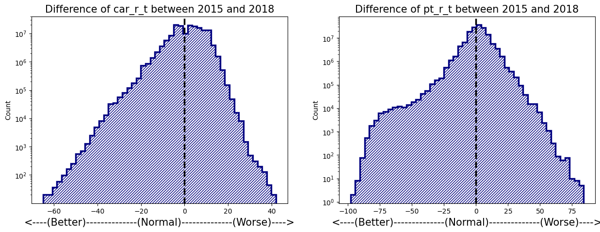
Difference between 2015 and 2018 dataset
- 각종 측면에서, 2015년 대비 2018년에 좋아지거나 또는 오히려 나빠진 Origin-Destion을 포착하고자 한다.
- 살펴볼 값의 대상은 아래 두 개를 선정했다.
- car_r_t: rush-hour(AM 8:00 ~ 9:00) 시간대 자가용 이용시 통행 소요 시간
- pt_r_t: rush-hour 시간대 대중교통 이용시 통행 소요 시간
1
2
3
4
5
6
7
8
9
10
11
12
13
14
15
16
17
18
19
20
21
22
23
24
25
26
27
28
29
30
31
32
33
34
35
36
DataPath = '/home/helsinki/helsinki_traveltime/dataset/'
parent_dirs = [file for file in os.listdir(DataPath) if not os.path.isfile(os.path.join(DataPath, file)) and file in ['2015', '2018']]
print(parent_dirs)

pt_r_t_matrix = np.zeros((13231, 13231, 2))
car_r_t_matrix = np.zeros((13231, 13231, 2))

firstFlag = True
for parent_idx, parent in tqdm(enumerate(parent_dirs)):
    child_dirs = [file for file in os.listdir(os.path.join(DataPath, parent)) if not os.path.isfile(os.path.join(DataPath, parent, file))]
    for child in child_dirs:
        babies = os.listdir(os.path.join(DataPath, parent, child))
        for i, baby in enumerate(babies):
            one_data = pd.read_csv(os.path.join(DataPath, parent, child, baby), sep=';')

            # to_id 가 전부 -1인 DataFrame도 있기에, .txt 파일명을 기준으로 destination YKR_ID를 추출한다.
            target_id = int(baby.split(' ')[1].split('.txt')[0])
            one_data = one_data.sort_values(by='from_id').reset_index(drop=True)
            if firstFlag:
                base_id_list = one_data['from_id'].values # 이 base_id_list 순서가 ndarray index의 기준이 된다.
                firstFlag = False
            else:
                if not np.array_equal(base_id_list, one_data['from_id'].values):
                    print(f"Ordering mis-matched with [base_id_list]: {parent}/{child}/{baby}")
                    continue # Should do in post-processing
                if target_id not in base_id_list:
                    print(f"Target ID not existed in [base_id_list]: {parent}/{child}/{baby}")
                    continue

            target_idx = np.argwhere(base_id_list==target_id)[0, 0]
            pt_r_t_matrix[:, target_idx, parent_idx] = one_data['pt_r_t'].values
            car_r_t_matrix[:, target_idx, parent_idx] = one_data['car_r_t'].values

# np.savetxt('BASE_ID_LIST.txt', base_id_list)
# np.save('pt_r_t_matrix_2018+2015.npy', pt_r_t_matrix)
# np.save('car_r_t_matrix_2018+2015.npy', car_r_t_matrix)
1
2
3
base_id_list = np.loadtxt('/home/helsinki/BASE_ID_LIST.txt')
car_r_t_matrix = np.load('/home/helsinki/car_r_t_matrix_2018+2015.npy')
pt_r_t_matrix = np.load('/home/helsinki/pt_r_t_matrix_2018+2015.npy')
1
2
3
4
5
6
7
def calculate_diff(ndarray):
    # Perform element-wise calculation, but only on non-zero and non-MinusOne values
    # 2018_result - 2015_result 계산을 수행할 때, 둘 중 한쪽이라도 0 또는 -1 값을 가지면 계산에서 제외시키고, 결과값 0으로 치환.
    valid_mask = (ndarray[:, :, 0] != 0) & (ndarray[:, :, 1] != 0) & (ndarray[:, :, 0] != -1) & (ndarray[:, :, 1] != -1)
    result = np.zeros_like(ndarray[:, :, 0])
    result[valid_mask] = ndarray[:, :, 0][valid_mask] - ndarray[:, :, 1][valid_mask]
    return result
1
2
3
4
5
6
7
diff_car_r_t = calculate_diff(car_r_t_matrix)
diff_car_flat = diff_car_r_t.flatten()
nonzero_car_diff = diff_car_flat[diff_car_flat != 0]

diff_pt_r_t = calculate_diff(pt_r_t_matrix)
diff_pt_flat = diff_pt_r_t.flatten()
nonzero_pt_diff = diff_pt_flat[diff_pt_flat != 0]
1
2
3
4
5
6
7
8
9
10
11
12
13
14
15
16
# Distribution of difference between 2015 and 2018
fig, axs = plt.subplots(nrows=1, ncols=2, facecolor='w', figsize=(15, 5))
axs[0].hist(nonzero_car_diff, bins=50, color='navy', histtype='step', hatch='//////', linewidth=2.5)
axs[0].axvline(0, color='black', linestyle='dashed', linewidth=2.5)
axs[0].set_yscale('log')
axs[0].set_xlabel("<----(Better)--------------(Normal)--------------(Worse)---->", fontsize=15)
axs[0].set_ylabel("Count")
axs[0].set_title("Difference of car_r_t between 2015 and 2018", fontsize=15)

axs[1].hist(nonzero_pt_diff, bins=50, color='navy', histtype='step', hatch='//////', linewidth=2.5)
axs[1].axvline(0, color='black', linestyle='dashed', linewidth=2.5)
axs[1].set_yscale('log')
axs[1].set_xlabel("<----(Better)--------------(Normal)--------------(Worse)---->", fontsize=15)
axs[1].set_ylabel("Count")
axs[1].set_title("Difference of pt_r_t between 2015 and 2018", fontsize=15)
plt.show()
1
2
3
4
5
6
7
8
# Embedding geographical position for all YKR Grids
node_pos_dict = defaultdict(list)
for _, row in tqdm(geojson_df.iterrows()):
    coords = row.centroid.xy
    lon, lat = coords[0][0], coords[1][0]
    node_pos_dict[row.YKR_ID] = [lon, lat]

    13231it [00:00, 13330.87it/s]
1
2
3
4
5
6
7
8
9
10
11
12
13
14
15
16
17
18
19
20
21
22
23
24
25
26
27
28
29
30
# Better OD / Worse OD 몇 개를 직접 그려보기 전에, Difference 값의 크기에 따라 edge width를 조절하고자 한다.
# MinMaxScaling을 통해 width의 차이를 emphasizing 할 생각이다.
def widths_with_SquareMinMaxScaling(G, min_width, max_width):
    """
    Given the instance of networkx(G), this function generates the widths of edges for drawing in future.
    The widths are calculated by the Square Min-Max Scaling method which is based on weights included in the G.

    Parameters
    ----------
    G : nx.graph
        All edges must have their own weights.
    min_width : int or float
        minimum width of edge
    max_width : int or float
        maximum width of edge

    Returns
    -------
    list
        the list for widths of edges, the orders follow the nx.graph (G).
    """
    widths = []
    weights = [G[s][t][0]['weight'] for s, t in G.edges()]
    min_w = np.min(weights)
    max_w = np.max(weights)
    for w in weights:
        wid = min_width + (max_width - min_width) * ((w - min_w) / (max_w - min_w)) ** 2
        widths.append(wid)

    return widths
1
2
3
4
5
6
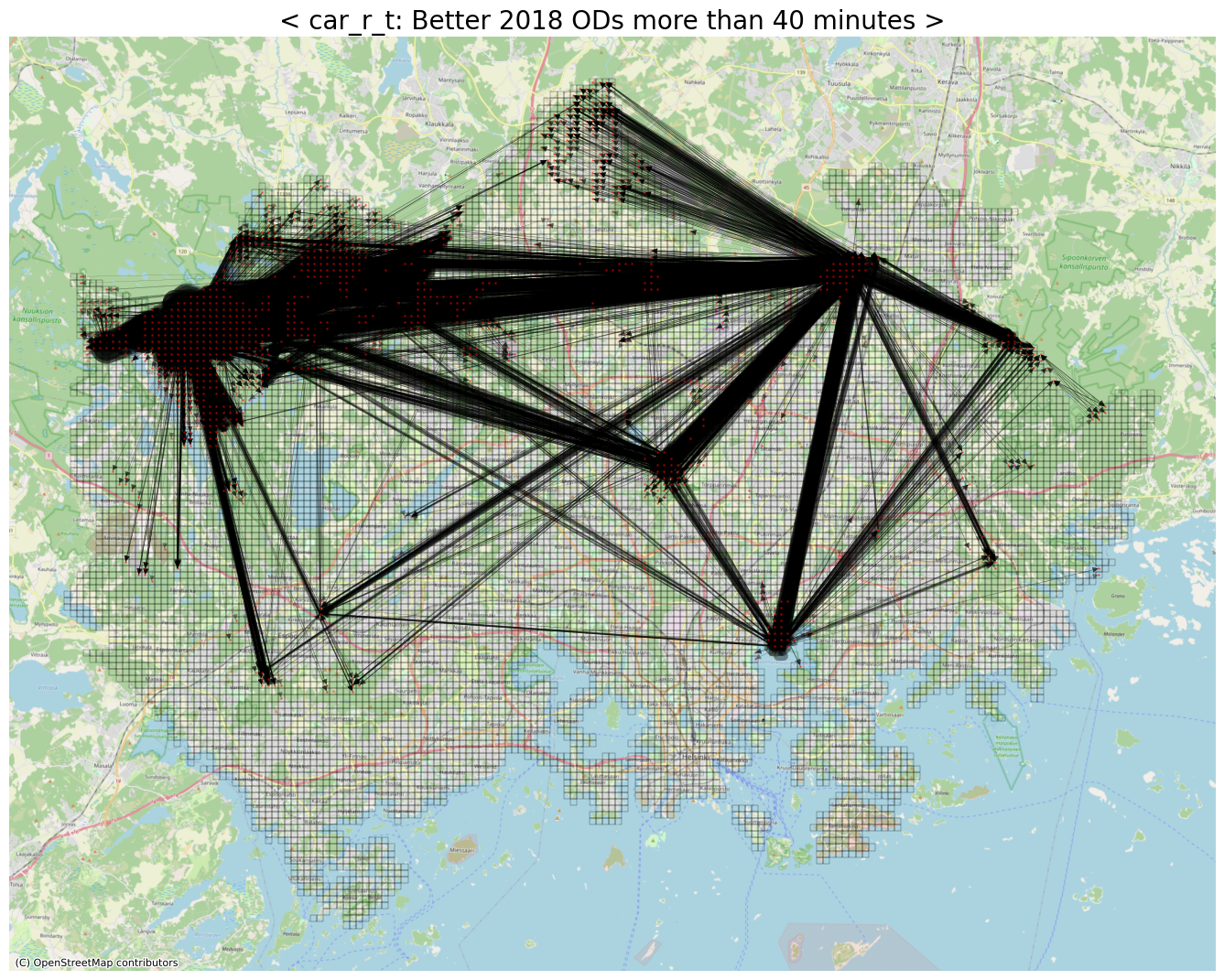
# Better ODs (with respect to car_r_t)
threshold = -40
row_idxs, col_idxs = np.where(diff_car_r_t < threshold) # rush-hour 시간대, 자가용 통행 소요 시간이 '40분 이상' 좋아진 OD들
print(f"The number of detected ODs: {row_idxs.shape[0]:,}")
The number of detected ODs: 7,658
1
2
3
4
5
6
7
8
9
10
11
target_weighted_edges = []
for row, col in tqdm(zip(row_idxs, col_idxs)):
    ykr_st, ykr_ed = base_id_list[row], base_id_list[col]
    weight = abs(diff_car_r_t[row, col])
    target_weighted_edges.append((int(ykr_st), int(ykr_ed), weight))

nxG = nx.MultiDiGraph()
nxG.add_weighted_edges_from(target_weighted_edges)
edge_widths = widths_with_SquareMinMaxScaling(nxG, min_width=0.1, max_width=25)

    7658it [00:00, 658155.85it/s]
1
2
3
4
5
6
7
fig, ax = plt.subplots(facecolor='w', figsize=(17, 17))
geojson_df.plot(ax=ax, facecolor='None', edgecolor='black', linewidth=.2)
cx.add_basemap(ax, crs=geojson_df.crs.to_string(), zoom=12, source=cx.providers.OpenStreetMap.Mapnik)
nx.draw_networkx(nxG, pos=node_pos_dict, with_labels=False, node_color='red', edge_color='black', node_size=1, alpha=.4, width=edge_widths, ax=ax)
ax.set_title(f"< car_r_t: Better 2018 ODs more than {abs(threshold)} minutes >", fontsize=20)
ax.axis('off')
plt.show()
1
2
3
4
5
6
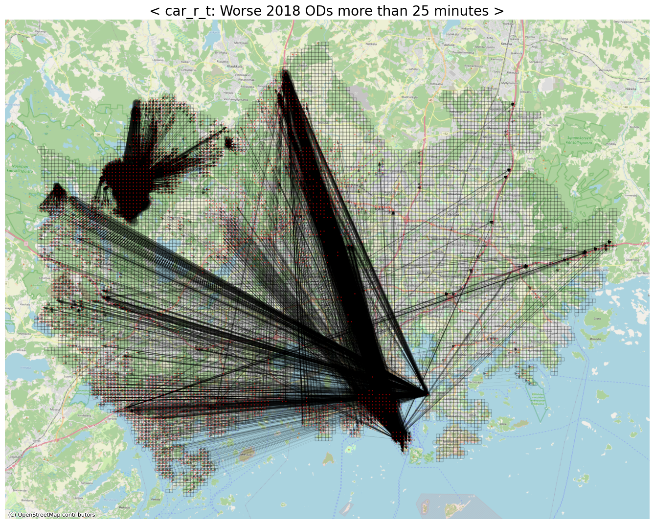
# Worse ODs (with respect to car_r_t)
threshold = 25
row_idxs, col_idxs = np.where(diff_car_r_t > threshold) # rush-hour 시간대, 자가용 통행 소요 시간이 '25분 이상' 안 좋아진 OD들
print(f"The number of detected ODs: {row_idxs.shape[0]:,}")
The number of detected ODs: 6,946
1
2
3
4
5
6
7
8
9
10
11
worse_car_weighted_edges = []
for row, col in tqdm(zip(row_idxs, col_idxs)):
    ykr_st, ykr_ed = base_id_list[row], base_id_list[col]
    weight = abs(diff_car_r_t[row, col])
    worse_car_weighted_edges.append((int(ykr_st), int(ykr_ed), weight))

nxG = nx.MultiDiGraph()
nxG.add_weighted_edges_from(worse_car_weighted_edges)
edge_widths = widths_with_SquareMinMaxScaling(nxG, min_width=0.1, max_width=25)

    6946it [00:00, 682590.28it/s]
1
2
3
4
5
6
7
fig, ax = plt.subplots(facecolor='w', figsize=(17, 17))
geojson_df.plot(ax=ax, facecolor='None', edgecolor='black', linewidth=.2)
cx.add_basemap(ax, crs=geojson_df.crs.to_string(), zoom=12, source=cx.providers.OpenStreetMap.Mapnik)
nx.draw_networkx(nxG, pos=node_pos_dict, with_labels=False, node_color='red', edge_color='black', node_size=1, alpha=.4, width=edge_widths, ax=ax)
ax.set_title(f"< car_r_t: Worse 2018 ODs more than {abs(threshold)} minutes >", fontsize=20)
ax.axis('off')
plt.show()
1
2
3
4
5
6
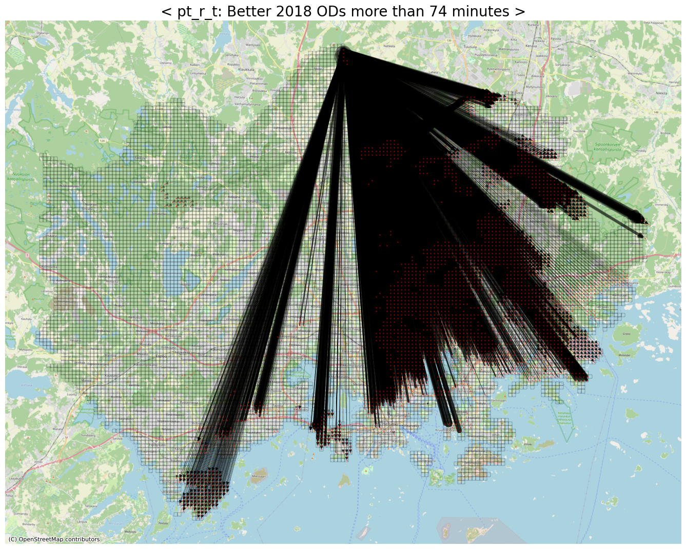
# Better ODs (with respect to pt_r_t)
threshold = -74
row_idxs, col_idxs = np.where(diff_pt_r_t < threshold)
print(f"The number of detected ODs: {row_idxs.shape[0]:,}")
The number of detected ODs: 8,214
1
2
3
4
5
6
7
8
9
10
11
pt_weighted_edges = []
for row, col in tqdm(zip(row_idxs, col_idxs)):
    ykr_st, ykr_ed = base_id_list[row], base_id_list[col]
    weight = abs(diff_pt_r_t[row, col])
    pt_weighted_edges.append((int(ykr_st), int(ykr_ed), weight))

nxG = nx.MultiDiGraph()
nxG.add_weighted_edges_from(pt_weighted_edges)
edge_widths = widths_with_SquareMinMaxScaling(nxG, min_width=0.1, max_width=25)

    8214it [00:00, 683802.34it/s]
1
2
3
4
5
6
7
fig, ax = plt.subplots(facecolor='w', figsize=(17, 17))
geojson_df.plot(ax=ax, facecolor='None', edgecolor='black', linewidth=.2)
cx.add_basemap(ax, crs=geojson_df.crs.to_string(), zoom=12, source=cx.providers.OpenStreetMap.Mapnik)
nx.draw_networkx(nxG, pos=node_pos_dict, with_labels=False, node_color='red', node_size=1, alpha=.4, width=edge_widths, ax=ax)
ax.set_title(f"< pt_r_t: Better 2018 ODs more than {abs(threshold)} minutes >", fontsize=20)
ax.axis('off')
plt.show()
1
2
3
4
5
6
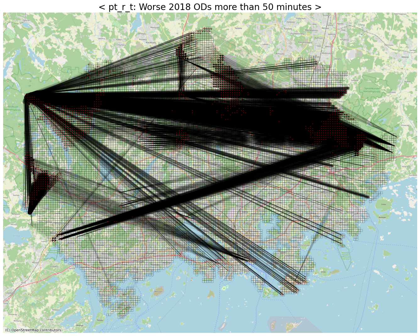
# Worse ODs (with respect to pt_r_t)
threshold = 50
row_idxs, col_idxs = np.where(diff_pt_r_t > threshold)
print(f"The number of detected ODs: {row_idxs.shape[0]:,}")
The number of detected ODs: 4,879
1
2
3
4
5
6
7
8
9
10
11
worse_pt_weighted_edges = []
for row, col in tqdm(zip(row_idxs, col_idxs)):
    ykr_st, ykr_ed = base_id_list[row], base_id_list[col]
    weight = abs(diff_pt_r_t[row, col])
    worse_pt_weighted_edges.append((int(ykr_st), int(ykr_ed), weight))

nxG = nx.MultiDiGraph()
nxG.add_weighted_edges_from(worse_pt_weighted_edges)
edge_widths = widths_with_SquareMinMaxScaling(nxG, min_width=0.1, max_width=25)

    4879it [00:00, 586697.51it/s]
1
2
3
4
5
6
7
fig, ax = plt.subplots(facecolor='w', figsize=(17, 17))
geojson_df.plot(ax=ax, facecolor='None', edgecolor='black', linewidth=.2)
cx.add_basemap(ax, crs=geojson_df.crs.to_string(), zoom=12, source=cx.providers.OpenStreetMap.Mapnik)
nx.draw_networkx(nxG, pos=node_pos_dict, with_labels=False, node_color='red', node_size=1, alpha=.4, width=edge_widths, ax=ax)
ax.set_title(f"< pt_r_t: Worse 2018 ODs more than {abs(threshold)} minutes >", fontsize=20)
ax.axis('off')
plt.show()
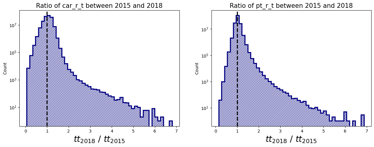
Ratio between 2015 and 2018
- 절대적 시간이 얼마나 줄거나 늘었는지 보는 관점은 OD간의 상대적인 거리에 따라 그 의미 자체에 바이어스가 있다는 생각이 든다.
- 예컨대, 서울에서 부산까지 가는 데 걸리는 시간이 30분 늘어난 상황과, 바로 옆동네 편의점을 들리는 데 30분 늘어난 상황이 체감적으로 다르듯이 말이다.
- 그래서 지리적으로/물리적으로 존재할 수 밖에 없는 소요 시간의 크기 스케일을 없애고자 비율로 다시 계산하여 시각화하였다.
1
2
3
4
5
6
7
def calculate_ratio(ndarray):
    # Perform element-wise calculation, but only on non-zero and non-MinusOne values
    # 2018_result vs. 2015_result 계산을 수행할 때, 둘 중 한쪽이라도 0 또는 -1 값을 가지면 계산에서 제외시키고, 최종 결과값 0으로 치환.
    valid_mask = (ndarray[:, :, 0] != 0) & (ndarray[:, :, 1] != 0) & (ndarray[:, :, 0] != -1) & (ndarray[:, :, 1] != -1)
    result = np.zeros_like(ndarray[:, :, 0])
    result[valid_mask] = ndarray[:, :, 0][valid_mask] / ndarray[:, :, 1][valid_mask]
    return result
1
2
3
4
5
6
7
diff_car_r_t = calculate_ratio(car_r_t_matrix)
diff_car_flat = diff_car_r_t.flatten()
nonzero_car_diff = diff_car_flat[diff_car_flat != 0]

diff_pt_r_t = calculate_ratio(pt_r_t_matrix)
diff_pt_flat = diff_pt_r_t.flatten()
nonzero_pt_diff = diff_pt_flat[diff_pt_flat != 0]
1
2
3
4
5
6
7
8
9
10
11
12
13
14
15
16
# Distribution of ratio between 2015 and 2018
fig, axs = plt.subplots(nrows=1, ncols=2, facecolor='w', figsize=(15, 5))
axs[0].hist(nonzero_car_diff, bins=50, color='navy', histtype='step', hatch='//////', linewidth=2.5)
axs[0].axvline(1, color='black', linestyle='dashed', linewidth=2.5)
axs[0].set_yscale('log')
axs[0].set_xlabel(r"$tt_{2018}$ / $tt_{2015}$", fontsize=20)
axs[0].set_ylabel("Count")
axs[0].set_title("Ratio of car_r_t between 2015 and 2018", fontsize=15)

axs[1].hist(nonzero_pt_diff, bins=50, color='navy', histtype='step', hatch='//////', linewidth=2.5)
axs[1].axvline(1, color='black', linestyle='dashed', linewidth=2.5)
axs[1].set_yscale('log')
axs[1].set_xlabel(r"$tt_{2018}$ / $tt_{2015}$", fontsize=20)
axs[1].set_ylabel("Count")
axs[1].set_title("Ratio of pt_r_t between 2015 and 2018", fontsize=15)
plt.show()
1
2
3
4
5
6
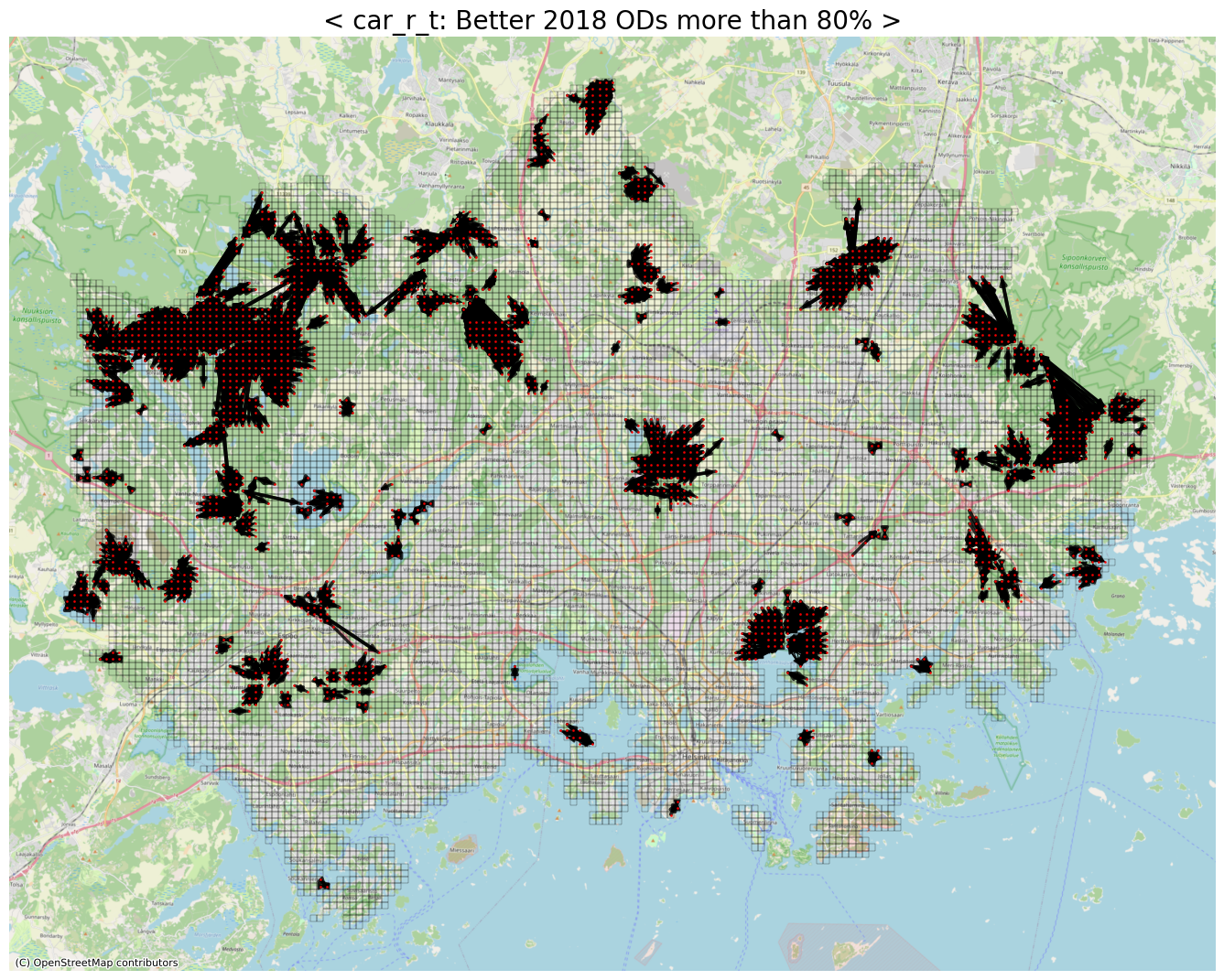
7
threshold = 0.2 # 2015년 대비 2018년에 80% 이상 좋아진 cases
print(threshold)
row_idxs, col_idxs = np.where(np.logical_and(diff_car_r_t > 0, diff_car_r_t < threshold)) # selfloop 는 0이기 때문에 제외
print(f"The number of detected ODs: {row_idxs.shape[0]:,}")
0.2
The number of detected ODs: 7,511
1
2
3
4
5
6
7
8
9
10
11
target_weighted_edges = []
for row, col in tqdm(zip(row_idxs, col_idxs)):
    ykr_st, ykr_ed = base_id_list[row], base_id_list[col]
    weight = abs(diff_car_r_t[row, col])
    target_weighted_edges.append((int(ykr_st), int(ykr_ed), weight))

nxG = nx.MultiDiGraph()
nxG.add_weighted_edges_from(target_weighted_edges)
edge_widths = widths_with_SquareMinMaxScaling(nxG, min_width=0.5, max_width=3)

    7511it [00:00, 663201.91it/s]
1
2
3
4
5
6
7
fig, ax = plt.subplots(facecolor='w', figsize=(17, 17))
geojson_df.plot(ax=ax, facecolor='None', edgecolor='black', linewidth=.2)
cx.add_basemap(ax, crs=geojson_df.crs.to_string(), zoom=12, source=cx.providers.OpenStreetMap.Mapnik)
nx.draw_networkx(nxG, pos=node_pos_dict, with_labels=False, node_color='red', edge_color='black', node_size=1, alpha=.8, width=edge_widths, ax=ax)
ax.set_title(f"< car_r_t: Better 2018 ODs more than {int((1-threshold)*100)}% >", fontsize=20)
ax.axis('off')
plt.show()
1
2
3
4
5
6
7
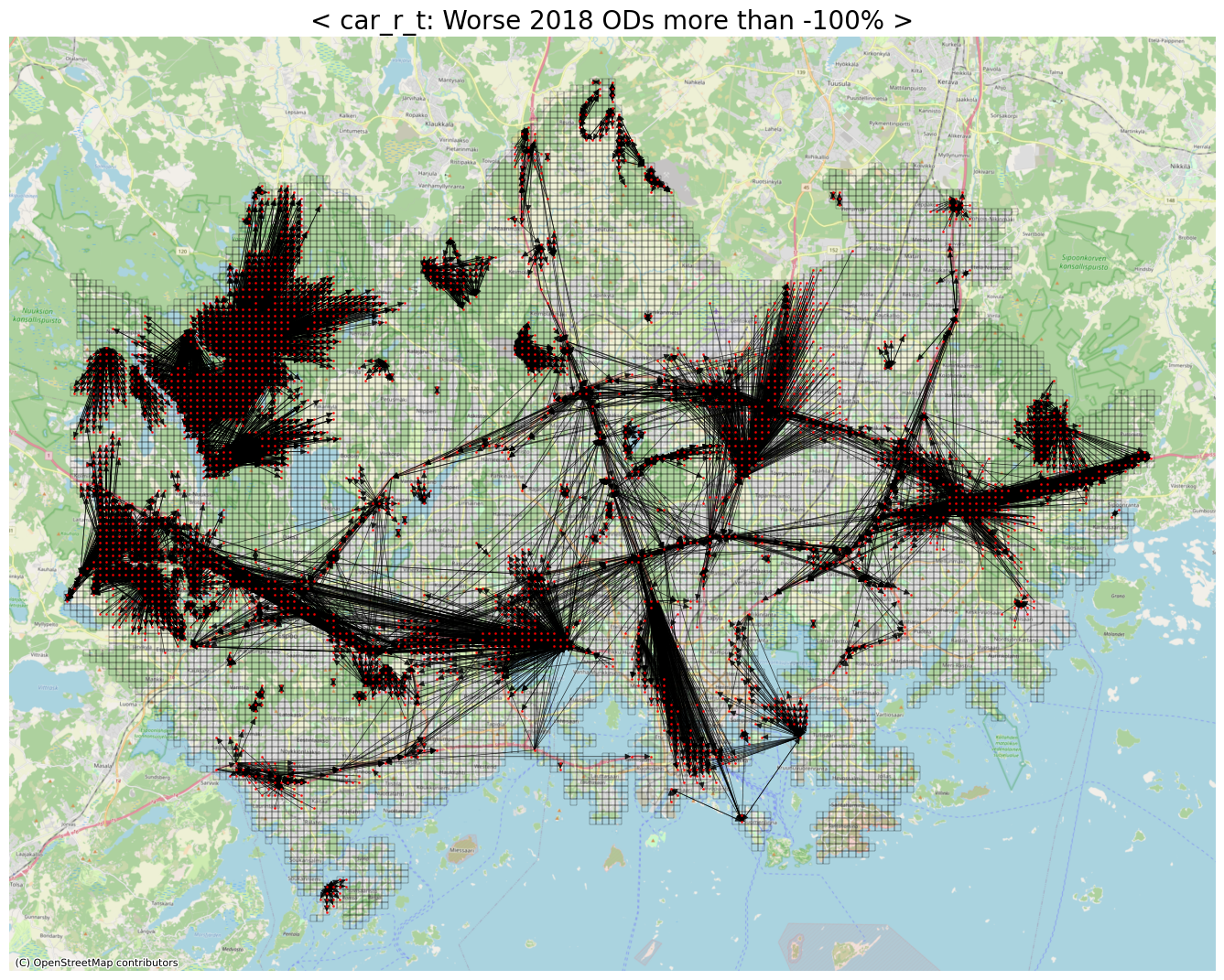
# Worse ODs (with respect to car_r_t)
# 기존보다 2배이상 (-100%) 안좋아진 OD들
threshold = 2
row_idxs, col_idxs = np.where(diff_car_r_t > threshold)
print(f"The number of detected ODs: {row_idxs.shape[0]:,}")
The number of detected ODs: 11,782
1
2
3
4
5
6
7
8
9
10
11
worse_car_weighted_edges = []
for row, col in tqdm(zip(row_idxs, col_idxs)):
    ykr_st, ykr_ed = base_id_list[row], base_id_list[col]
    weight = abs(diff_car_r_t[row, col])
    worse_car_weighted_edges.append((int(ykr_st), int(ykr_ed), weight))

nxG = nx.MultiDiGraph()
nxG.add_weighted_edges_from(worse_car_weighted_edges)
edge_widths = widths_with_SquareMinMaxScaling(nxG, min_width=0.5, max_width=3)

    11782it [00:00, 696567.57it/s]
1
2
3
4
5
6
7
fig, ax = plt.subplots(facecolor='w', figsize=(17, 17))
geojson_df.plot(ax=ax, facecolor='None', edgecolor='black', linewidth=.2)
cx.add_basemap(ax, crs=geojson_df.crs.to_string(), zoom=12, source=cx.providers.OpenStreetMap.Mapnik)
nx.draw_networkx(nxG, pos=node_pos_dict, with_labels=False, node_color='red', edge_color='black', node_size=1, alpha=.8, width=edge_widths, ax=ax)
ax.set_title(f"< car_r_t: Worse 2018 ODs more than {int((1-threshold)*100)}% >", fontsize=20)
ax.axis('off')
plt.show()
1
2
3
4
5
6
7
8
9
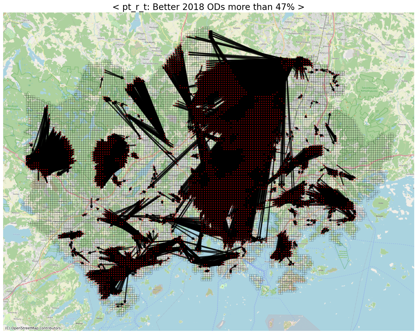
# 'pt_r_t' version
# 2015년 대비 2018년에 47% 이상 좋아진 cases
threshold = 0.53
print(threshold)
row_idxs, col_idxs = np.where(np.logical_and(diff_pt_r_t > 0, diff_pt_r_t < threshold)) # selfloop 는 0이기 때문에 제외
print(f"The number of detected ODs: {row_idxs.shape[0]:,}")
0.53
The number of detected ODs: 11,222
1
2
3
4
5
6
7
8
9
10
11
pt_weighted_edges = []
for row, col in tqdm(zip(row_idxs, col_idxs)):
    ykr_st, ykr_ed = base_id_list[row], base_id_list[col]
    weight = abs(diff_pt_r_t[row, col])
    pt_weighted_edges.append((int(ykr_st), int(ykr_ed), weight))

nxG = nx.MultiDiGraph()
nxG.add_weighted_edges_from(pt_weighted_edges)
edge_widths = widths_with_SquareMinMaxScaling(nxG, min_width=0.5, max_width=3)

    11222it [00:00, 713299.28it/s]
1
2
3
4
5
6
7
fig, ax = plt.subplots(facecolor='w', figsize=(17, 17))
geojson_df.plot(ax=ax, facecolor='None', edgecolor='black', linewidth=.2)
cx.add_basemap(ax, crs=geojson_df.crs.to_string(), zoom=12, source=cx.providers.OpenStreetMap.Mapnik)
nx.draw_networkx(nxG, pos=node_pos_dict, with_labels=False, node_color='red', node_size=1, alpha=.8, width=edge_widths, ax=ax)
ax.set_title(f"< pt_r_t: Better 2018 ODs more than {int(round(1-threshold, 2)*100)}% >", fontsize=20)
ax.axis('off')
plt.show()
1
2
3
4
5
6
7
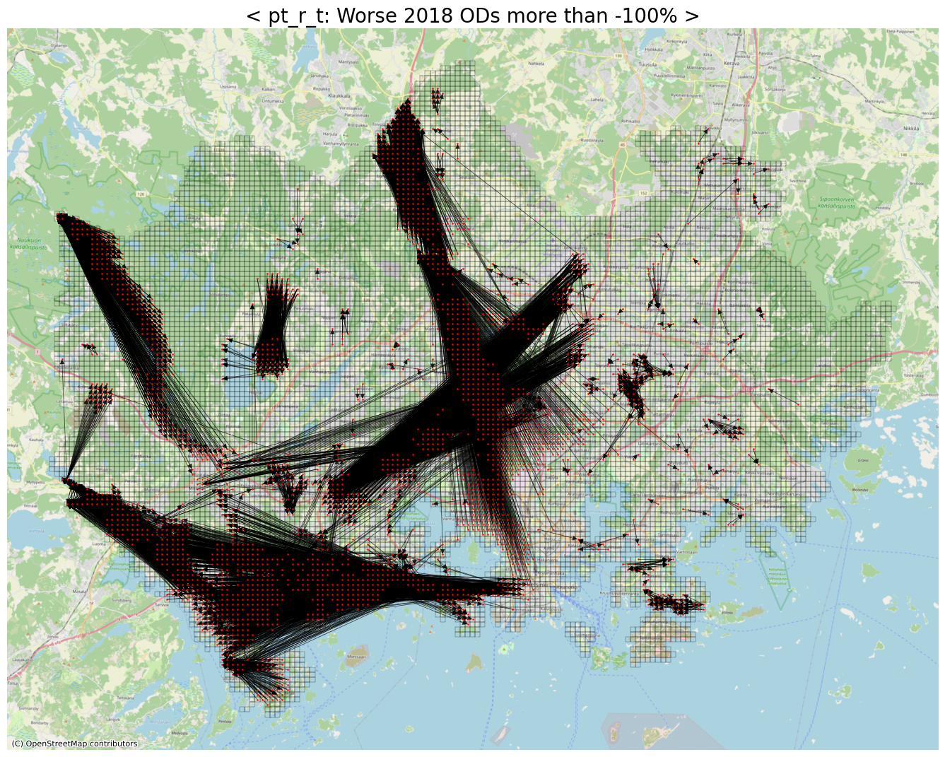
# Worse ODs
# 기존보다 2배이상 (-100%) 안좋아진 OD들
threshold = 2
row_idxs, col_idxs = np.where(diff_pt_r_t > threshold)
print(f"The number of detected ODs: {row_idxs.shape[0]:,}")
The number of detected ODs: 13,869
1
2
3
4
5
6
7
8
9
10
11
worse_pt_weighted_edges = []
for row, col in tqdm(zip(row_idxs, col_idxs)):
    ykr_st, ykr_ed = base_id_list[row], base_id_list[col]
    weight = abs(diff_pt_r_t[row, col])
    worse_pt_weighted_edges.append((int(ykr_st), int(ykr_ed), weight))

nxG = nx.MultiDiGraph()
nxG.add_weighted_edges_from(worse_pt_weighted_edges)
edge_widths = widths_with_SquareMinMaxScaling(nxG, min_width=0.5, max_width=3)

    13869it [00:00, 730211.04it/s]
1
2
3
4
5
6
7
fig, ax = plt.subplots(facecolor='w', figsize=(17, 17))
geojson_df.plot(ax=ax, facecolor='None', edgecolor='black', linewidth=.2)
cx.add_basemap(ax, crs=geojson_df.crs.to_string(), zoom=12, source=cx.providers.OpenStreetMap.Mapnik)
nx.draw_networkx(nxG, pos=node_pos_dict, with_labels=False, node_color='red', node_size=1, alpha=.8, width=edge_widths, ax=ax)
ax.set_title(f"< pt_r_t: Worse 2018 ODs more than {int(round(1-threshold, 2)*100)}% >", fontsize=20)
ax.axis('off')
plt.show()
Take-Home Message and Discussion
- 핀란드의 수도 헬싱키의 통행시간 데이터를 살펴보았다.
- 2013년, 2015년, 2018년 연단위로 집계된 데이터셋이다.
- walk, cycling, public transport, car 각각에 대해서 따로 travel time이 기록되어 있다.
- 유의사항 1: Attribute(column)의 종류 수 측면에서, 2018 > 2015 > 2013 이다.
- 유의사항 2: 납득이 안가는 0 또는 -1 같은 이상치들이 존재한다.
- origin과 destination이 명시되어 있어서, OD matrix 기반의 network analysis를 수행할 수 있다.
- YKR Grid 라는 핀란드 정부에서 정의한 250m by 250m 크기의 grd를 사용하고 있다. (헬싱키에 속하는 YKR Grid는 총 13,231개)
- 본 작업에서는 car_r_t 및 pt_r_t 측면에서, 2015년 대비 2018년에 좋아지거나 안좋아진 OD들을 살펴보았다.
- Distribution of difference
- Network Drawing for Better or Worse ODs
- Ratio (Travel Time of 2018 / Travel Time of 2015)
fin