들어가며
오늘은 SafeGraph Inc.에서 재가공 및 공개 배포 중인 Open Census Data를 살펴본 내용이다. 본 데이터는 사실 US Census Bureau에서 이미 배포 중인 각종 demographic 데이터들을 하나로 종합해 정리한 데이터라고 보면 된다. 지역별 인구수, 소득 수준 같은 속성 뿐 아니라, 특정 시설수 같은 정보도 포함되어 있다.
US Census Bureau(미국 인구조사국) 는 다양한 특성에 대한 다양한 인구통계적(demographic) 정보를 조사 및 수집하는 기관이다. 대표적인 ‘국내 인구수 조사(Census)’도 이런 여러 demographic data 중 하나이다. Census 조사는 보통 대규모의 인력과 비용, 그리고 시간이 요구되기 때문에, 미국같은 경우는 10년마다 모집단 조사(full survey)를 수행하고 결과를 발표한다. 이게 이른바, Decennial Census라고 부르는 공식 결과다. 그리고 미국 인구조사국은 이 외에도 지역마다의 성별수(Gender), 나이(Age), 소득(Income), 민족계통(Ethnicity; 라틴아메리카(히스패닉계) or 아시아계 or 아프리카계 or 유럽계) 등을 조사한다. 이 조사는 American Community Survey; ACS라는 프로젝트 이름으로 매년 샘플링 조사(sample survey)를 통해 집계하여 결과를 발표한다.
SafeGraph - Open Census Data
1
2
3
4
5
6
7
8
import os
import numpy as np
import pandas as pd
import matplotlib.pyplot as plt
import gdown
from tqdm import tqdm
import tarfile
import geopandas as gpd
Data Acquisition
현재 배포되고 있는 데이터들의 Google Drive 고유파일 ID와 파일이름들을 정리해뒀다.
1
2
3
4
5
6
7
8
9
# File ID and Name
IDnFN = [['1klKXB35iXyhfbgKTEXZXgdhZWJDwpbEi', 'safegraph_open_census_data_2020.tar.gz'], \
    ['1v2MTZG9MNW-ao8fSeO6r69AfHsXB2mwx', 'safegraph_open_census_data_2020_to_2029_geometry.tar.gz'], \
    ['1rMF7doWkgoKvAs4GPi5FpQNhOFd9V9b2', 'safegraph_open_census_data_2020_redistricting.tar.gz'], \
    ['1ab-dGzzDntCEE8wVBekAQpvsOZvxSbVV', 'safegraph_open_census_data_2019.tar.gz'], \
    ['1oUT_UBUCa6nRZ207taXHAeANmpHEwsGt', 'safegraph_open_census_data_2018.tar.gz'], \
    ['15TFKFONZquET0AvpFlsENSOP2dk2w39V', 'safegraph_open_census_data_2017.tar.gz'], \
    ['10InSSafTPUZ6tK-e8g6msYepCO9i2H3L', 'safegraph_open_census_data_2016.tar.gz'], \
    ['1QmKe7v7peaYAjDDh50hNP4b9s0B0JTWm', 'safegraph_open_census_data_2010_to_2019_geometry.tar.gz']]
1
2
3
4
gdrive_base_path = 'https://drive.google.com/uc?id='
SavePath = '/open_census_data'
for file_id, file_name in tqdm(IDnFN):
    gdown.download(gdrive_base_path + file_id, os.path.join(SavePath, file_name), quiet=True)
1
100%|██████████| 8/8 [04:37<00:00, 34.67s/it]
1
2
3
4
5
6
7
# unzip 'safegraph_open_census_data_2020.tar.gz'
with tarfile.open(os.path.join(SavePath, IDnFN[0][1]), 'r:gz') as tr:
    tr.extractall(path=SavePath)

# unzip 'safegraph_open_census_data_2020_to_2029_geometry.tar.gz' to extract a geojson file of 'cbg_2020.geojson'
with tarfile.open(os.path.join(SavePath, IDnFN[1][1]), 'r:gz') as tr:
    tr.extractall(path=SavePath)
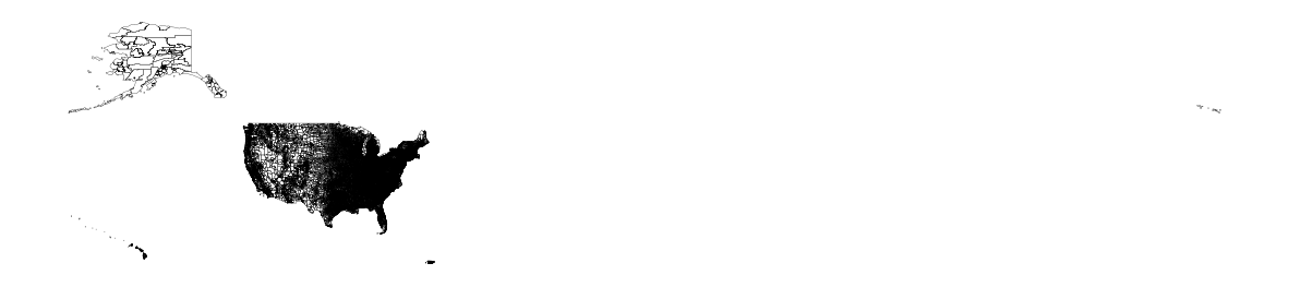
US Census GeoJson
US Census Bureau의 집계 단위인 Census Block Group(cbg)의 polygon-styled and geometrical GeoJSON 파일이다. 용량이 커서(~1.9 GB) 불러오는데 꽤 시간이 소요된다. Polygon-style로 시각화 할 게 아니면, 각 census data 내의 ‘/metadata/cbg_geographic_data.csv’를 사용하자.
1
2
3
4
5
BasePath = '/open_census_data'
FileContents = os.listdir(BasePath)

cbg_geo = gpd.read_file(os.path.join(BasePath, FileContents[1]))
cbg_geo
| StateFIPS | CountyFIPS | TractCode | BlockGroup | CensusBlockGroup | State | County | MTFCC | geometry | |
|---|---|---|---|---|---|---|---|---|---|
| 0 | 01 | 033 | 020200 | 1 | 010330202001 | AL | Colbert County | G5030 | MULTIPOLYGON (((-87.70081 34.76189, -87.70081 ... |
| 1 | 01 | 019 | 956000 | 1 | 010199560001 | AL | Cherokee County | G5030 | MULTIPOLYGON (((-85.67917 34.15255, -85.67904 ... |
| 2 | 01 | 073 | 004701 | 2 | 010730047012 | AL | Jefferson County | G5030 | MULTIPOLYGON (((-86.78478 33.51157, -86.78267 ... |
| 3 | 01 | 073 | 004702 | 1 | 010730047021 | AL | Jefferson County | G5030 | MULTIPOLYGON (((-86.77400 33.51790, -86.77396 ... |
| 4 | 01 | 073 | 004702 | 2 | 010730047022 | AL | Jefferson County | G5030 | MULTIPOLYGON (((-86.77621 33.50359, -86.77599 ... |
| ... | ... | ... | ... | ... | ... | ... | ... | ... | ... |
| 242330 | 72 | 127 | 008300 | 3 | 721270083003 | PR | San Juan Municipio | G5030 | MULTIPOLYGON (((-66.09123 18.39897, -66.08954 ... |
| 242331 | 72 | 127 | 010012 | 3 | 721270100123 | PR | San Juan Municipio | G5030 | MULTIPOLYGON (((-66.04081 18.36705, -66.04076 ... |
| 242332 | 72 | 127 | 010022 | 2 | 721270100222 | PR | San Juan Municipio | G5030 | MULTIPOLYGON (((-66.05515 18.37903, -66.05482 ... |
| 242333 | 72 | 127 | 010100 | 1 | 721270101001 | PR | San Juan Municipio | G5030 | MULTIPOLYGON (((-66.07215 18.34087, -66.07208 ... |
| 242334 | 72 | 127 | 010100 | 3 | 721270101003 | PR | San Juan Municipio | G5030 | MULTIPOLYGON (((-66.08014 18.32918, -66.08002 ... |
242335 rows × 9 columns
1
2
3
4
fig, ax = plt.subplots(facecolor='w', figsize=(15, 15))
cbg_geo.plot(ax=ax, facecolor='None', edgecolor='black', linewidth=0.2)
ax.axis('off')
plt.show()
이 글에선 미국 본토 내 “48개 주 + District of Columbia; 즉 워싱턴 D.C“만을 다룬다.
한 가지 TMI,,, 미국 자체는 크게 3계층 구조를 지닌다고 한다.
- United States: 50개 states + 워싱턴 D.C (미국 수도인 워싱턴 D.C는 어느 주에도 속하지 않음)
- Continental United States: ‘하와이주’를 제외한 49개 states + 워싱턴 D.C
- Conterminous/Contiguous United States: ‘하와이주’와 ‘알래스카주’를 제외한 48개 states + 워싱턴 D.C
즉, Conterminous(Contiguous) United States 만 다루겠다는 말이다.
두 번째 TMI,,, ‘하와이주’와 ‘알래스카주’를 제외한 48개 states를 Lower 48 states라고 부르기도 한다고 한다.
1
2
# 하와이주(HI), 알래스카주(AK) + 푸에르토리코(PR)까지 총 3개 제외
us_cbg_geo = cbg_geo[~cbg_geo['State'].isin(['AK', 'HI', 'PR'])].reset_index(drop=True)
1
2
3
4
fig, ax = plt.subplots(facecolor='w', figsize=(15, 15))
us_cbg_geo.plot(ax=ax, facecolor='None', edgecolor='black', linewidth=0.2)
ax.axis('off')
plt.show()
US Open Census Data
2023년 6월 기준, SafeGraph에서 재가공-배포 중인 demographic dataset은 다음과 같다.
- 2016 5-year ACS : 2012.01 ~ 2016.12까지의 매해 ACS의 결과를 평균 집계한 데이터
- 2017 5-year ACS : 2013.01 ~ 2017.12 ACS 평균 집계
- 2018 5-year ACS : 2014.01 ~ 2018.12 ACS 평균 집계
- 2019 5-year ACS : 2015.01 ~ 2019.12 ACS 평균 집계
- 2010-2019 Census Block Group geometries : 2010년 ~ 2019년 사이 데이터들의 집계 기준으로 활용한 GeoJSON
- (NEW) 2020 5-year ACS : 2016.01 ~ 2020.12
- (NEW) 2020-2029 Census Block Group geometries : 2020년 ~ 2029년 사이 데이터들의 집계 기준으로 활용할 GeoJSON
- (NEW) 2020 decennial redistricting data : 2020년판 Decennial Survey (미국 인구총조사 발표 데이터; 인구수에 대한 데이터만 있음; ACS 아님)
참고로, 엄밀히 말하자면, 5년 묶음으로 취합 및 집계한 이 데이터들(Multiyear dataset)도 US Census Bureau 측에서 ACS 일환으로 수행한 자료이다. 자세한 내용이 궁금하다면 아래 미국 인구조사국 공식 홈페이지 내용을 참고하자.
https://www.census.gov/programs-surveys/acs/guidance/estimates.html
: ‘When to Use 1-year or 5-year Estimates’ by US Census Bureau
https://www2.census.gov/programs-surveys/acs/tech_docs/accuracy/MultiyearACSAccuracyofData2019.pdf
: ‘Detailed of multiyear(5-year) Dataset’ by US Census Bureau
그러면 SafeGraph Inc. 측 홈페이지에 데이터 업로드의 취지와 목적이 궁금할 수 있는데, 그들은 아래와 같이 설명하고 있다.
“While the US Census Bureau offers free downloads of their data, it’s often difficult and confusing to get bulk access to it at the granularity needed for advanced analysis.
(Therefore) We’ve pre-cleaned this data and packaged it into easy to use…“
- SafeGraph Inc. (https://www.safegraph.com/free-data/open-census-data).
대충 정리하자면, 미국 인구 조사국에서 올려놓은 ACS 각종 자료들이 여기저기 흩어져있고 사용자들의 접근과 활용이 어려우니, 더욱 사용이 용이하게끔 우리가 잘 정리해서 재배포한다는 취지이다. 아무튼 그렇다. 아무튼 이 글에서 나는 SafeGraph’s <2020 5-year ACS> 데이터(아래 Dataset Structure 참고)를 살펴보도록 한다.
1
2
3
4
5
6
7
8
9
10
11
safegraph_open_census_data_2020
├── data
│   ├── cbg_b01.csv     # field 명으로 데이터들이 나눠져있다. (field: household income, median age, population etc...)
│   ├── cbg_b02.csv
│   ├── ...
│   ├── ...
│   └── cbg_c24.csv
└── metadata
    ├── cbg_field_descriptions.csv          # field 들에 대한 설명
    ├── cbg_fips_codes.csv                  # us fips code
    └── cbg_geographic_data.csv             # point-styled CBG geometry (longitude and latitude)
데이터에 포함된 모든 속성의 테이블 정의서는 여기 미국 인구조사국 사이트에서 열람할 수 있다.
1
2
3
4
BasePath = '/open_census_data/safegraph_open_census_data_2020'
SubDir = os.listdir(BasePath)
cbg_fd_desc = pd.read_csv(os.path.join(BasePath, SubDir[1], 'cbg_field_descriptions.csv'))
cbg_fd_desc.head()
| table_id | table_number | table_title | table_topics | table_universe | field_level_1 | field_level_2 | field_level_3 | field_level_4 | field_level_5 | field_level_6 | field_level_7 | field_level_8 | field_level_9 | field_level_10 | |
|---|---|---|---|---|---|---|---|---|---|---|---|---|---|---|---|
| 0 | B01001e1 | B01001 | Sex By Age | Age and Sex | Total population | Estimate | SEX BY AGE | Total population | Total | NaN | NaN | NaN | NaN | NaN | NaN |
| 1 | B01001e10 | B01001 | Sex By Age | Age and Sex | Total population | Estimate | SEX BY AGE | Total population | Total | Male | 22 to 24 years | NaN | NaN | NaN | NaN |
| 2 | B01001e11 | B01001 | Sex By Age | Age and Sex | Total population | Estimate | SEX BY AGE | Total population | Total | Male | 25 to 29 years | NaN | NaN | NaN | NaN |
| 3 | B01001e12 | B01001 | Sex By Age | Age and Sex | Total population | Estimate | SEX BY AGE | Total population | Total | Male | 30 to 34 years | NaN | NaN | NaN | NaN |
| 4 | B01001e13 | B01001 | Sex By Age | Age and Sex | Total population | Estimate | SEX BY AGE | Total population | Total | Male | 35 to 39 years | NaN | NaN | NaN | NaN |
1
2
3
4
# field_level_1 에는 크게 'Estimate'과 'MarginOfError'에 해당하는 field가 있다.
# 이 글에선 측정치(값) 자체만 보고자 하므로 'Estimate'으로만 관심 field 수를 제한하겠다.
cbg_fd_desc = cbg_fd_desc[cbg_fd_desc['field_level_1']=='Estimate'].reset_index(drop=True)
cbg_fd_desc
| table_id | table_number | table_title | table_topics | table_universe | field_level_1 | field_level_2 | field_level_3 | field_level_4 | field_level_5 | field_level_6 | field_level_7 | field_level_8 | field_level_9 | field_level_10 | |
|---|---|---|---|---|---|---|---|---|---|---|---|---|---|---|---|
| 0 | B01001e1 | B01001 | Sex By Age | Age and Sex | Total population | Estimate | SEX BY AGE | Total population | Total | NaN | NaN | NaN | NaN | NaN | NaN |
| 1 | B01001e10 | B01001 | Sex By Age | Age and Sex | Total population | Estimate | SEX BY AGE | Total population | Total | Male | 22 to 24 years | NaN | NaN | NaN | NaN |
| 2 | B01001e11 | B01001 | Sex By Age | Age and Sex | Total population | Estimate | SEX BY AGE | Total population | Total | Male | 25 to 29 years | NaN | NaN | NaN | NaN |
| 3 | B01001e12 | B01001 | Sex By Age | Age and Sex | Total population | Estimate | SEX BY AGE | Total population | Total | Male | 30 to 34 years | NaN | NaN | NaN | NaN |
| 4 | B01001e13 | B01001 | Sex By Age | Age and Sex | Total population | Estimate | SEX BY AGE | Total population | Total | Male | 35 to 39 years | NaN | NaN | NaN | NaN |
| ... | ... | ... | ... | ... | ... | ... | ... | ... | ... | ... | ... | ... | ... | ... | ... |
| 4077 | C24030e55 | C24030 | Sex By Industry For The Civilian Employed Popu... | Age and Sex, Civilian Population, Industry | Civilian employed population 16 years and over | Estimate | SEX BY INDUSTRY FOR THE CIVILIAN EMPLOYED POPU... | Civilian employed population 16 years and over | Total | Female | Public administration | NaN | NaN | NaN | NaN |
| 4078 | C24030e6 | C24030 | Sex By Industry For The Civilian Employed Popu... | Age and Sex, Civilian Population, Industry | Civilian employed population 16 years and over | Estimate | SEX BY INDUSTRY FOR THE CIVILIAN EMPLOYED POPU... | Civilian employed population 16 years and over | Total | Male | Construction | NaN | NaN | NaN | NaN |
| 4079 | C24030e7 | C24030 | Sex By Industry For The Civilian Employed Popu... | Age and Sex, Civilian Population, Industry | Civilian employed population 16 years and over | Estimate | SEX BY INDUSTRY FOR THE CIVILIAN EMPLOYED POPU... | Civilian employed population 16 years and over | Total | Male | Manufacturing | NaN | NaN | NaN | NaN |
| 4080 | C24030e8 | C24030 | Sex By Industry For The Civilian Employed Popu... | Age and Sex, Civilian Population, Industry | Civilian employed population 16 years and over | Estimate | SEX BY INDUSTRY FOR THE CIVILIAN EMPLOYED POPU... | Civilian employed population 16 years and over | Total | Male | Wholesale trade | NaN | NaN | NaN | NaN |
| 4081 | C24030e9 | C24030 | Sex By Industry For The Civilian Employed Popu... | Age and Sex, Civilian Population, Industry | Civilian employed population 16 years and over | Estimate | SEX BY INDUSTRY FOR THE CIVILIAN EMPLOYED POPU... | Civilian employed population 16 years and over | Total | Male | Retail trade | NaN | NaN | NaN | NaN |
4082 rows × 15 columns
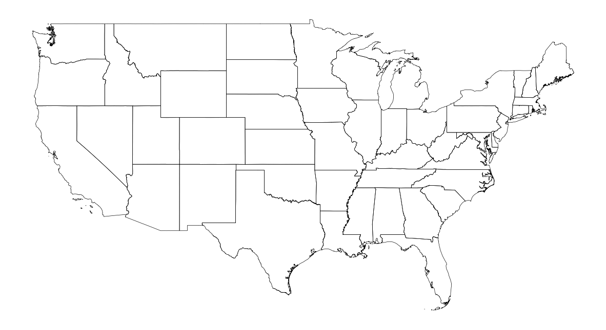
Alternative for US and CBG Geometry
CBG Geometries GeoJSON 파일은 다루기 너무 무거워서, State-level의 다른 shapefiles(cb_2018_us_state_500k)을 찾아 사용하였다. 아래 URL 참조.
https://www.census.gov/geographies/mapping-files/time-series/geo/carto-boundary-file.html
1
2
3
4
# Load Point-styled CBG geometry
cbg_geo_lonlat = pd.read_csv(os.path.join(BasePath, SubDir[1], 'cbg_geographic_data.csv'))
# cbg_geo_lonlat['census_block_group'] = cbg_geo_lonlat['census_block_group'].apply(lambda x: f"{x:012d}") # 자릿수맞추기: CBG 코드는 12글자
cbg_geo_lonlat.head()
| census_block_group | amount_land | amount_water | latitude | longitude | |
|---|---|---|---|---|---|
| 0 | 10010201001 | 4264299 | 28435 | 32.465832 | -86.489661 |
| 1 | 10010201002 | 5561005 | 0 | 32.485873 | -86.489672 |
| 2 | 10010202001 | 2058374 | 0 | 32.480082 | -86.474974 |
| 3 | 10010202002 | 1262444 | 5669 | 32.464435 | -86.469766 |
| 4 | 10010203001 | 3866513 | 9054 | 32.480175 | -86.460792 |
1
2
3
4
5
6
7
us_states = gpd.read_file('/open_census_data/cb_2018_us_state_500k')
us_states = us_states[~us_states['STUSPS'].isin(['PR', 'AK', 'HI', 'AS', 'VI', 'GU', 'MP'])]

fig, ax = plt.subplots(facecolor='w', figsize=(15, 15))
us_states.plot(ax=ax, facecolor='None', edgecolor='black', linewidth=.5)
ax.axis('off')
plt.show()
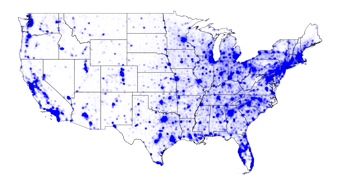
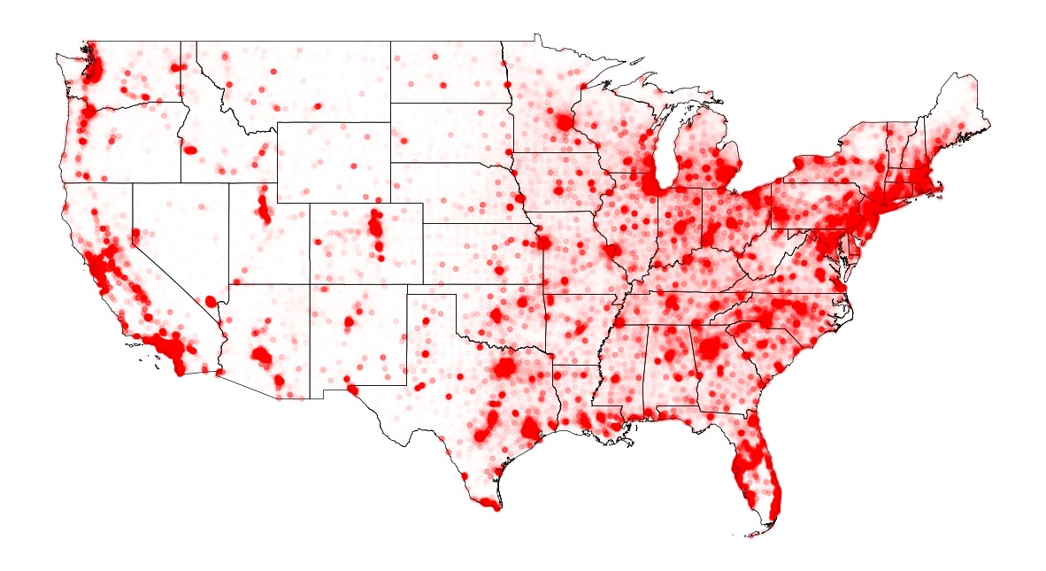
Gender Population for each CBG
- table_id(male) = B01001e2
- table_id(female) = B01001e26
1
cbg_fd_desc[cbg_fd_desc['table_id'].isin(['B01001e2', 'B01001e26'])]
| table_id | table_number | table_title | table_topics | table_universe | field_level_1 | field_level_2 | field_level_3 | field_level_4 | field_level_5 | field_level_6 | field_level_7 | field_level_8 | field_level_9 | field_level_10 | |
|---|---|---|---|---|---|---|---|---|---|---|---|---|---|---|---|
| 11 | B01001e2 | B01001 | Sex By Age | Age and Sex | Total population | Estimate | SEX BY AGE | Total population | Total | Male | NaN | NaN | NaN | NaN | NaN |
| 18 | B01001e26 | B01001 | Sex By Age | Age and Sex | Total population | Estimate | SEX BY AGE | Total population | Total | Female | NaN | NaN | NaN | NaN | NaN |
1
2
3
4
5
# table_number 앞 세자리를 따서 /data에서 파일을 찾아 불러온다.
BasePath = '/open_census_data/safegraph_open_census_data_2020'
print(os.path.join(BasePath, SubDir[0]))
cbg_b01 = pd.read_csv(os.path.join(BasePath, SubDir[0], 'cbg_b01.csv'))
cbg_b01.head()
1
/open_census_data/safegraph_open_census_data_2020/data
| census_block_group | B01001e1 | B01001m1 | B01001e2 | B01001m2 | B01001e3 | B01001m3 | B01001e4 | B01001m4 | B01001e5 | ... | B01002He3 | B01002Hm3 | B01002Ie1 | B01002Im1 | B01002Ie2 | B01002Im2 | B01002Ie3 | B01002Im3 | B01003e1 | B01003m1 | |
|---|---|---|---|---|---|---|---|---|---|---|---|---|---|---|---|---|---|---|---|---|---|
| 0 | 10010201001 | 674 | 192 | 284 | 88 | 12 | 15 | 17 | 23 | 5 | ... | 37.5 | 27.2 | NaN | NaN | NaN | NaN | NaN | NaN | 674 | 192 |
| 1 | 10010201002 | 1267 | 401 | 694 | 244 | 49 | 65 | 80 | 88 | 45 | ... | 35.0 | 5.6 | NaN | NaN | NaN | NaN | NaN | NaN | 1267 | 401 |
| 2 | 10010202001 | 706 | 200 | 354 | 142 | 50 | 38 | 72 | 69 | 15 | ... | 28.8 | 4.2 | 65.8 | 37.6 | NaN | NaN | 65.8 | 37.6 | 706 | 200 |
| 3 | 10010202002 | 1051 | 229 | 656 | 175 | 31 | 26 | 5 | 9 | 7 | ... | 42.3 | 10.0 | NaN | NaN | NaN | NaN | NaN | NaN | 1051 | 229 |
| 4 | 10010203001 | 2912 | 565 | 1461 | 289 | 22 | 23 | 134 | 69 | 200 | ... | 35.7 | 2.8 | 28.0 | 22.1 | 27.6 | 0.5 | 28.9 | 58.7 | 2912 | 565 |
5 rows × 161 columns
1
2
3
4
5
6
cbg_b01 = pd.merge(cbg_b01, cbg_geo_lonlat, on='census_block_group')
cbg_b01 = gpd.GeoDataFrame(cbg_b01, geometry=gpd.points_from_xy(cbg_b01.longitude, cbg_b01.latitude))
cbg_b01 = cbg_b01.set_crs(epsg=4269) # The EPSG of 'cb_2018_us_state_500k' is 4269. But note that EPSG of CBG_geojson is 4326.

# gpd.sjoin(how='left/right/inner/'): ‘inner’: use intersection of keys from both dfs; retain only left_df geometry column
cbg_b01 = gpd.sjoin(cbg_b01, us_states[['NAME', 'geometry']], how='inner') # Spatial Join based on the Lower 48 states
1
2
3
4
5
6
7
8
9
10
11
12
13
14
15
16
17
18
19
20
def alpha_with_SquareMinMaxScaling(values, min_alpha, max_alpha):
    """
    min_alpha : int or float
        minimum alpha for color
    max_alpha : int or float
        maximum alpha for color

    Returns
    -------
    Sequential list
        the alpha list for each value, the order must be controlled carefully.
    """
    alphas = []
    min_val = np.min(values)
    max_val = np.max(values)
    for v in values:
        alp = min_alpha + (max_alpha - min_alpha) * ((v - min_val) / (max_val - min_val)) ** 2
        alphas.append(alp)

    return alphas
1
2
3
4
5
6
7
8
9
cbg_gender_pop = cbg_b01.loc[:, ['census_block_group', 'longitude', 'latitude', 'B01001e2', 'B01001e26']].rename(columns={'B01001e2':'male', 'B01001e26':'female'})

# Only Male
male_alps = alpha_with_SquareMinMaxScaling(cbg_gender_pop['male'].values, 0.01, 0.85)
fig, ax = plt.subplots(facecolor='w', figsize=(15, 15))
us_states.plot(ax=ax, facecolor='None', edgecolor='black', linewidth=.5)
ax.scatter(cbg_gender_pop['longitude'], cbg_gender_pop['latitude'], s=15, c='blue', alpha=male_alps)
ax.axis('off')
plt.show()
1
2
3
4
5
6
7
# Only Female
female_alps = alpha_with_SquareMinMaxScaling(cbg_gender_pop['female'].values, 0.01, 0.85)
fig, ax = plt.subplots(facecolor='w', figsize=(15, 15))
us_states.plot(ax=ax, facecolor='None', edgecolor='black', linewidth=.5)
ax.scatter(cbg_gender_pop['longitude'], cbg_gender_pop['latitude'], s=15, c='red', alpha=female_alps)
ax.axis('off')
plt.show()
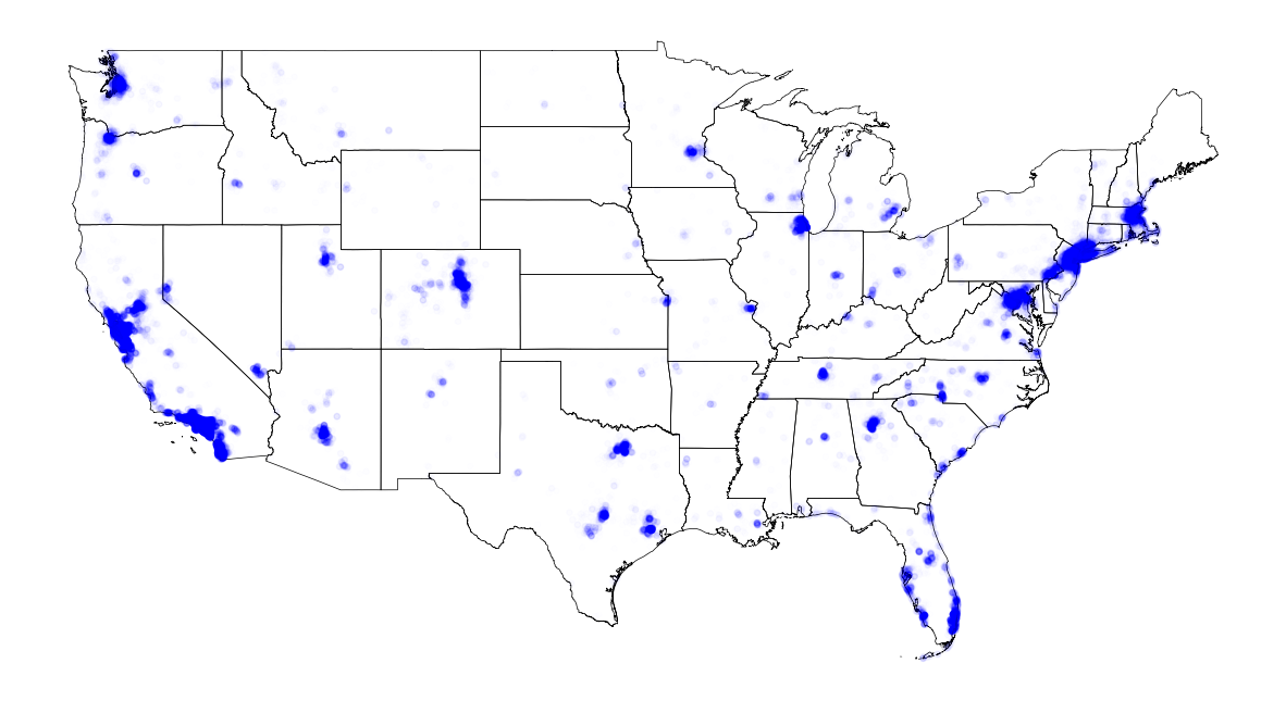
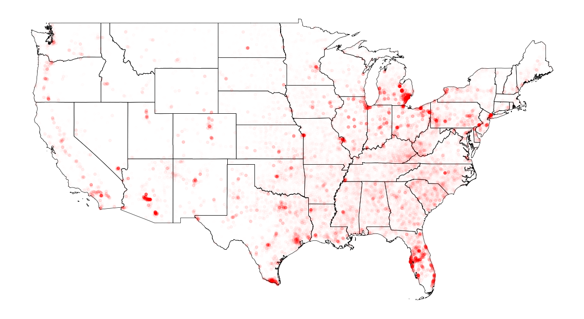
The Number of House by Housing Value for each CBG
부동산 가치가 높은 지역과 낮은 지역이 어디인지 살펴본다. 임의의 금액 기준을 두고, 해당하는 field 인덱스들을 찾아 분류했다.
- $500,000 이상 table_id: B25075e23, B25075e24, B25075e25, B25075e26, B25075e27
- $50,000 미만 table_id: B25075e2, B25075e3, B25075e4, B25075e5, B25075e6, B25075e7, B25075e8, B25075e9
1
2
cntHouse_fd_desc = cbg_fd_desc[cbg_fd_desc['table_title']=='Value'].reset_index(drop=True)
cntHouse_fd_desc
| table_id | table_number | table_title | table_topics | table_universe | field_level_1 | field_level_2 | field_level_3 | field_level_4 | field_level_5 | field_level_6 | field_level_7 | field_level_8 | field_level_9 | field_level_10 | |
|---|---|---|---|---|---|---|---|---|---|---|---|---|---|---|---|
| 0 | B25075e1 | B25075 | Value | Housing Value and Purchase Price, Owner Renter... | Owner-occupied housing units | Estimate | VALUE | Owner-occupied housing units | Total | NaN | NaN | NaN | NaN | NaN | NaN |
| 1 | B25075e10 | B25075 | Value | Housing Value and Purchase Price, Owner Renter... | Owner-occupied housing units | Estimate | VALUE | Owner-occupied housing units | Total | $50 000 to $59 999 | NaN | NaN | NaN | NaN | NaN |
| 2 | B25075e11 | B25075 | Value | Housing Value and Purchase Price, Owner Renter... | Owner-occupied housing units | Estimate | VALUE | Owner-occupied housing units | Total | $60 000 to $69 999 | NaN | NaN | NaN | NaN | NaN |
| 3 | B25075e12 | B25075 | Value | Housing Value and Purchase Price, Owner Renter... | Owner-occupied housing units | Estimate | VALUE | Owner-occupied housing units | Total | $70 000 to $79 999 | NaN | NaN | NaN | NaN | NaN |
| 4 | B25075e13 | B25075 | Value | Housing Value and Purchase Price, Owner Renter... | Owner-occupied housing units | Estimate | VALUE | Owner-occupied housing units | Total | $80 000 to $89 999 | NaN | NaN | NaN | NaN | NaN |
| 5 | B25075e14 | B25075 | Value | Housing Value and Purchase Price, Owner Renter... | Owner-occupied housing units | Estimate | VALUE | Owner-occupied housing units | Total | $90 000 to $99 999 | NaN | NaN | NaN | NaN | NaN |
| 6 | B25075e15 | B25075 | Value | Housing Value and Purchase Price, Owner Renter... | Owner-occupied housing units | Estimate | VALUE | Owner-occupied housing units | Total | $100 000 to $124 999 | NaN | NaN | NaN | NaN | NaN |
| 7 | B25075e16 | B25075 | Value | Housing Value and Purchase Price, Owner Renter... | Owner-occupied housing units | Estimate | VALUE | Owner-occupied housing units | Total | $125 000 to $149 999 | NaN | NaN | NaN | NaN | NaN |
| 8 | B25075e17 | B25075 | Value | Housing Value and Purchase Price, Owner Renter... | Owner-occupied housing units | Estimate | VALUE | Owner-occupied housing units | Total | $150 000 to $174 999 | NaN | NaN | NaN | NaN | NaN |
| 9 | B25075e18 | B25075 | Value | Housing Value and Purchase Price, Owner Renter... | Owner-occupied housing units | Estimate | VALUE | Owner-occupied housing units | Total | $175 000 to $199 999 | NaN | NaN | NaN | NaN | NaN |
| 10 | B25075e19 | B25075 | Value | Housing Value and Purchase Price, Owner Renter... | Owner-occupied housing units | Estimate | VALUE | Owner-occupied housing units | Total | $200 000 to $249 999 | NaN | NaN | NaN | NaN | NaN |
| 11 | B25075e2 | B25075 | Value | Housing Value and Purchase Price, Owner Renter... | Owner-occupied housing units | Estimate | VALUE | Owner-occupied housing units | Total | Less than $10 000 | NaN | NaN | NaN | NaN | NaN |
| 12 | B25075e20 | B25075 | Value | Housing Value and Purchase Price, Owner Renter... | Owner-occupied housing units | Estimate | VALUE | Owner-occupied housing units | Total | $250 000 to $299 999 | NaN | NaN | NaN | NaN | NaN |
| 13 | B25075e21 | B25075 | Value | Housing Value and Purchase Price, Owner Renter... | Owner-occupied housing units | Estimate | VALUE | Owner-occupied housing units | Total | $300 000 to $399 999 | NaN | NaN | NaN | NaN | NaN |
| 14 | B25075e22 | B25075 | Value | Housing Value and Purchase Price, Owner Renter... | Owner-occupied housing units | Estimate | VALUE | Owner-occupied housing units | Total | $400 000 to $499 999 | NaN | NaN | NaN | NaN | NaN |
| 15 | B25075e23 | B25075 | Value | Housing Value and Purchase Price, Owner Renter... | Owner-occupied housing units | Estimate | VALUE | Owner-occupied housing units | Total | $500 000 to $749 999 | NaN | NaN | NaN | NaN | NaN |
| 16 | B25075e24 | B25075 | Value | Housing Value and Purchase Price, Owner Renter... | Owner-occupied housing units | Estimate | VALUE | Owner-occupied housing units | Total | $750 000 to $999 999 | NaN | NaN | NaN | NaN | NaN |
| 17 | B25075e25 | B25075 | Value | Housing Value and Purchase Price, Owner Renter... | Owner-occupied housing units | Estimate | VALUE | Owner-occupied housing units | Total | $1 000 000 to $1 499 999 | NaN | NaN | NaN | NaN | NaN |
| 18 | B25075e26 | B25075 | Value | Housing Value and Purchase Price, Owner Renter... | Owner-occupied housing units | Estimate | VALUE | Owner-occupied housing units | Total | $1 500 000 to $1 999 999 | NaN | NaN | NaN | NaN | NaN |
| 19 | B25075e27 | B25075 | Value | Housing Value and Purchase Price, Owner Renter... | Owner-occupied housing units | Estimate | VALUE | Owner-occupied housing units | Total | $2 000 000 or more | NaN | NaN | NaN | NaN | NaN |
| 20 | B25075e3 | B25075 | Value | Housing Value and Purchase Price, Owner Renter... | Owner-occupied housing units | Estimate | VALUE | Owner-occupied housing units | Total | $10 000 to $14 999 | NaN | NaN | NaN | NaN | NaN |
| 21 | B25075e4 | B25075 | Value | Housing Value and Purchase Price, Owner Renter... | Owner-occupied housing units | Estimate | VALUE | Owner-occupied housing units | Total | $15 000 to $19 999 | NaN | NaN | NaN | NaN | NaN |
| 22 | B25075e5 | B25075 | Value | Housing Value and Purchase Price, Owner Renter... | Owner-occupied housing units | Estimate | VALUE | Owner-occupied housing units | Total | $20 000 to $24 999 | NaN | NaN | NaN | NaN | NaN |
| 23 | B25075e6 | B25075 | Value | Housing Value and Purchase Price, Owner Renter... | Owner-occupied housing units | Estimate | VALUE | Owner-occupied housing units | Total | $25 000 to $29 999 | NaN | NaN | NaN | NaN | NaN |
| 24 | B25075e7 | B25075 | Value | Housing Value and Purchase Price, Owner Renter... | Owner-occupied housing units | Estimate | VALUE | Owner-occupied housing units | Total | $30 000 to $34 999 | NaN | NaN | NaN | NaN | NaN |
| 25 | B25075e8 | B25075 | Value | Housing Value and Purchase Price, Owner Renter... | Owner-occupied housing units | Estimate | VALUE | Owner-occupied housing units | Total | $35 000 to $39 999 | NaN | NaN | NaN | NaN | NaN |
| 26 | B25075e9 | B25075 | Value | Housing Value and Purchase Price, Owner Renter... | Owner-occupied housing units | Estimate | VALUE | Owner-occupied housing units | Total | $40 000 to $49 999 | NaN | NaN | NaN | NaN | NaN |
1
2
3
4
5
# table_number 앞 세자리를 따서 /data에서 파일을 찾아 불러온다.
BasePath = '/open_census_data/safegraph_open_census_data_2020'
print(os.path.join(BasePath, SubDir[0]))
cbg_b25 = pd.read_csv(os.path.join(BasePath, SubDir[0], 'cbg_b25.csv'))
cbg_b25.head()
1
/open_census_data/safegraph_open_census_data_2020/data
| census_block_group | B25001e1 | B25001m1 | B25002e1 | B25002m1 | B25002e2 | B25002m2 | B25002e3 | B25002m3 | B25003e1 | ... | B25093e25 | B25093m25 | B25093e26 | B25093m26 | B25093e27 | B25093m27 | B25093e28 | B25093m28 | B25093e29 | B25093m29 | |
|---|---|---|---|---|---|---|---|---|---|---|---|---|---|---|---|---|---|---|---|---|---|
| 0 | 10010201001 | 290 | 77 | 290 | 77 | 290 | 77 | 0 | 12 | 290 | ... | 7 | 8 | 18 | 31 | 15 | 23 | 12 | 21 | 0 | 12 |
| 1 | 10010201002 | 420 | 116 | 420 | 116 | 403 | 113 | 17 | 27 | 403 | ... | 0 | 12 | 4 | 6 | 0 | 12 | 3 | 6 | 0 | 12 |
| 2 | 10010202001 | 284 | 57 | 284 | 57 | 227 | 53 | 57 | 49 | 227 | ... | 3 | 5 | 11 | 17 | 0 | 12 | 0 | 12 | 0 | 12 |
| 3 | 10010202002 | 436 | 83 | 436 | 83 | 346 | 86 | 90 | 52 | 346 | ... | 17 | 17 | 0 | 12 | 0 | 12 | 2 | 4 | 0 | 12 |
| 4 | 10010203001 | 1147 | 185 | 1147 | 185 | 1034 | 185 | 113 | 89 | 1034 | ... | 0 | 12 | 4 | 7 | 5 | 8 | 22 | 26 | 0 | 12 |
5 rows × 1741 columns
1
2
3
4
cbg_b25 = pd.merge(cbg_b25, cbg_geo_lonlat, on='census_block_group')
cbg_b25 = gpd.GeoDataFrame(cbg_b25, geometry=gpd.points_from_xy(cbg_b25.longitude, cbg_b25.latitude))
cbg_b25 = cbg_b25.set_crs(epsg=4269)
cbg_b25 = gpd.sjoin(cbg_b25, us_states[['NAME', 'geometry']], how='inner').reset_index(drop=True) # Spatial Join based on the Lower 48 states
1
cbg_b25.head()
| census_block_group | B25001e1 | B25001m1 | B25002e1 | B25002m1 | B25002e2 | B25002m2 | B25002e3 | B25002m3 | B25003e1 | ... | B25093m28 | B25093e29 | B25093m29 | amount_land | amount_water | latitude | longitude | geometry | index_right | NAME | |
|---|---|---|---|---|---|---|---|---|---|---|---|---|---|---|---|---|---|---|---|---|---|
| 0 | 10010201001 | 290 | 77 | 290 | 77 | 290 | 77 | 0 | 12 | 290 | ... | 21 | 0 | 12 | 4264299 | 28435 | 32.465832 | -86.489661 | POINT (-86.48966 32.46583) | 17 | Alabama |
| 1 | 10010201002 | 420 | 116 | 420 | 116 | 403 | 113 | 17 | 27 | 403 | ... | 6 | 0 | 12 | 5561005 | 0 | 32.485873 | -86.489672 | POINT (-86.48967 32.48587) | 17 | Alabama |
| 2 | 10010202001 | 284 | 57 | 284 | 57 | 227 | 53 | 57 | 49 | 227 | ... | 12 | 0 | 12 | 2058374 | 0 | 32.480082 | -86.474974 | POINT (-86.47497 32.48008) | 17 | Alabama |
| 3 | 10010202002 | 436 | 83 | 436 | 83 | 346 | 86 | 90 | 52 | 346 | ... | 4 | 0 | 12 | 1262444 | 5669 | 32.464435 | -86.469766 | POINT (-86.46977 32.46444) | 17 | Alabama |
| 4 | 10010203001 | 1147 | 185 | 1147 | 185 | 1034 | 185 | 113 | 89 | 1034 | ... | 26 | 0 | 12 | 3866513 | 9054 | 32.480175 | -86.460792 | POINT (-86.46079 32.48018) | 17 | Alabama |
5 rows × 1748 columns
1
2
HighMortValue = 'B25075e23, B25075e24, B25075e25, B25075e26, B25075e27'.split(', ')
LowMortValue = 'B25075e2, B25075e3, B25075e4, B25075e5, B25075e6, B25075e7, B25075e8, B25075e9'.split(', ')
1
2
3
cbg_cntHouse_value = cbg_b25.loc[:, ['census_block_group', 'latitude', 'longitude']]
cbg_cntHouse_value['HighHouseCnt'] = cbg_b25.loc[:, HighMortValue].sum(axis=1)
cbg_cntHouse_value['LowHouseCnt'] = cbg_b25.loc[:, LowMortValue].sum(axis=1)
1
2
3
4
5
6
7
# The number of House with high value (more than $500,000)
high_alps = alpha_with_SquareMinMaxScaling(cbg_cntHouse_value['HighHouseCnt'].values, 0, 0.85)
fig, ax = plt.subplots(facecolor='w', figsize=(15, 15))
us_states.plot(ax=ax, facecolor='None', edgecolor='black', linewidth=.5)
ax.scatter(cbg_cntHouse_value['longitude'], cbg_cntHouse_value['latitude'], s=15, c='blue', alpha=high_alps)
ax.axis('off')
plt.show()
1
2
3
4
5
6
7
# The number of House with low value (lower than $50,000)
low_alps = alpha_with_SquareMinMaxScaling(cbg_cntHouse_value['LowHouseCnt'].values, 0, 0.85)
fig, ax = plt.subplots(facecolor='w', figsize=(15, 15))
us_states.plot(ax=ax, facecolor='None', edgecolor='black', linewidth=.5)
ax.scatter(cbg_cntHouse_value['longitude'], cbg_cntHouse_value['latitude'], s=15, c='red', alpha=low_alps)
ax.axis('off')
plt.show()
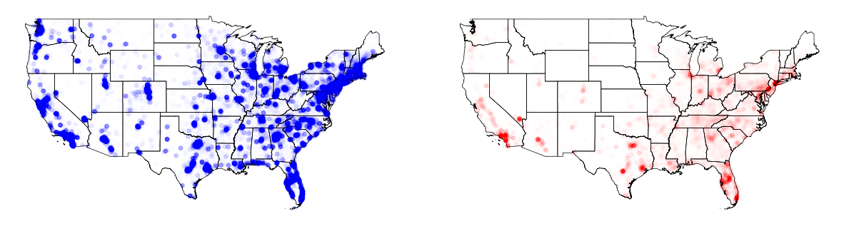
Educational Attainment for only US citizens 18 years and over
교육 수준이 높고, 낮은 인구가 미국 어디에 몰려있는지 살펴본다.
- 초중고 중퇴 및 고졸 table_id: B29002e2, B29002e3, B29002e4
- 전문대 졸(Associate’s degree), 일반대 졸(Bachelor’s degree) 및 석사이상 table_id: B29002e6, B29002e7, B29002e8
1
2
3
4
5
# table_number 앞 세자리를 따서 /data에서 파일을 찾아 불러온다.
BasePath = '/open_census_data/safegraph_open_census_data_2020'
print(os.path.join(BasePath, SubDir[0]))
cbg_b29 = pd.read_csv(os.path.join(BasePath, SubDir[0], 'cbg_b29.csv'))
cbg_b29.head()
1
/open_census_data/safegraph_open_census_data_2020/data
| census_block_group | B29001e1 | B29001m1 | B29001e2 | B29001m2 | B29001e3 | B29001m3 | B29001e4 | B29001m4 | B29001e5 | ... | B29002e8 | B29002m8 | B29003e1 | B29003m1 | B29003e2 | B29003m2 | B29003e3 | B29003m3 | B29004e1 | B29004m1 | |
|---|---|---|---|---|---|---|---|---|---|---|---|---|---|---|---|---|---|---|---|---|---|
| 0 | 10010201001 | 574 | 161 | 102 | 81 | 120 | 79 | 226 | 77 | 126 | ... | 55 | 35 | 574 | 161 | 72 | 63 | 502 | 164 | 39167.0 | 20140.0 |
| 1 | 10010201002 | 948 | 256 | 163 | 80 | 298 | 130 | 322 | 134 | 165 | ... | 76 | 34 | 948 | 256 | 100 | 70 | 848 | 245 | 70699.0 | 11633.0 |
| 2 | 10010202001 | 458 | 121 | 89 | 52 | 143 | 67 | 103 | 40 | 123 | ... | 7 | 9 | 458 | 121 | 106 | 66 | 352 | 108 | 39750.0 | 20003.0 |
| 3 | 10010202002 | 974 | 211 | 289 | 143 | 223 | 83 | 301 | 73 | 161 | ... | 37 | 27 | 762 | 201 | 39 | 37 | 723 | 204 | 50221.0 | 3210.0 |
| 4 | 10010203001 | 2045 | 413 | 317 | 131 | 730 | 234 | 680 | 221 | 318 | ... | 172 | 98 | 2045 | 413 | 170 | 93 | 1875 | 412 | 66843.0 | 10424.0 |
5 rows × 35 columns
1
2
target_table = 'B29002e2, B29002e3, B29002e4, B29002e6, B29002e7, B29002e8'.split(', ')
target_table
1
['B29002e2', 'B29002e3', 'B29002e4', 'B29002e6', 'B29002e7', 'B29002e8']
1
cbg_fd_desc[cbg_fd_desc['table_id'].isin(target_table)].reset_index(drop=True)
| table_id | table_number | table_title | table_topics | table_universe | field_level_1 | field_level_2 | field_level_3 | field_level_4 | field_level_5 | field_level_6 | field_level_7 | field_level_8 | field_level_9 | field_level_10 | |
|---|---|---|---|---|---|---|---|---|---|---|---|---|---|---|---|
| 0 | B29002e2 | B29002 | Citizen, Voting-Age Population By Educational ... | Age and Sex, Citizenship, Educational Attainment | Citizens 18 years and over | Estimate | CITIZEN, VOTING-AGE POPULATION BY EDUCATIONAL ... | Citizens 18 years and over | Total | Less than 9th grade | NaN | NaN | NaN | NaN | NaN |
| 1 | B29002e3 | B29002 | Citizen, Voting-Age Population By Educational ... | Age and Sex, Citizenship, Educational Attainment | Citizens 18 years and over | Estimate | CITIZEN, VOTING-AGE POPULATION BY EDUCATIONAL ... | Citizens 18 years and over | Total | 9th to 12th grade no diploma | NaN | NaN | NaN | NaN | NaN |
| 2 | B29002e4 | B29002 | Citizen, Voting-Age Population By Educational ... | Age and Sex, Citizenship, Educational Attainment | Citizens 18 years and over | Estimate | CITIZEN, VOTING-AGE POPULATION BY EDUCATIONAL ... | Citizens 18 years and over | Total | High school graduate (includes equivalency) | NaN | NaN | NaN | NaN | NaN |
| 3 | B29002e6 | B29002 | Citizen, Voting-Age Population By Educational ... | Age and Sex, Citizenship, Educational Attainment | Citizens 18 years and over | Estimate | CITIZEN, VOTING-AGE POPULATION BY EDUCATIONAL ... | Citizens 18 years and over | Total | Associate's degree | NaN | NaN | NaN | NaN | NaN |
| 4 | B29002e7 | B29002 | Citizen, Voting-Age Population By Educational ... | Age and Sex, Citizenship, Educational Attainment | Citizens 18 years and over | Estimate | CITIZEN, VOTING-AGE POPULATION BY EDUCATIONAL ... | Citizens 18 years and over | Total | Bachelor's degree | NaN | NaN | NaN | NaN | NaN |
| 5 | B29002e8 | B29002 | Citizen, Voting-Age Population By Educational ... | Age and Sex, Citizenship, Educational Attainment | Citizens 18 years and over | Estimate | CITIZEN, VOTING-AGE POPULATION BY EDUCATIONAL ... | Citizens 18 years and over | Total | Graduate or professional degree | NaN | NaN | NaN | NaN | NaN |
1
2
3
4
cbg_b29 = pd.merge(cbg_b29, cbg_geo_lonlat, on='census_block_group')
cbg_b29 = gpd.GeoDataFrame(cbg_b29, geometry=gpd.points_from_xy(cbg_b29.longitude, cbg_b29.latitude))
cbg_b29 = cbg_b29.set_crs(epsg=4269)
cbg_b29 = gpd.sjoin(cbg_b29, us_states[['NAME', 'geometry']], how='inner').reset_index(drop=True) # Spatial Join based on the Lower 48 states
1
2
3
4
5
6
HighEdu = 'B29002e6, B29002e7, B29002e8'.split(', ')
LowEdu = 'B29002e2, B29002e3, B29002e4'.split(', ')

cbg_cntPop_edu = cbg_b29.loc[:, ['census_block_group', 'latitude', 'longitude']]
cbg_cntPop_edu['HighEduPop'] = cbg_b29.loc[:, HighEdu].sum(axis=1)
cbg_cntPop_edu['LowEduPop'] = cbg_b29.loc[:, LowEdu].sum(axis=1)
1
2
3
4
5
6
7
8
9
10
11
12
13
14
15
# The number of House with high value (more than $500,000)
high_alps = alpha_with_SquareMinMaxScaling(cbg_cntPop_edu['HighEduPop'].values, 0, 0.85)
low_alps = alpha_with_SquareMinMaxScaling(cbg_cntPop_edu['LowEduPop'].values, 0, 0.85)

fig, axs = plt.subplots(nrows=1, ncols=2, facecolor='w', figsize=(15, 15))
us_states.plot(ax=axs[0], facecolor='None', edgecolor='black', linewidth=.5)
us_states.plot(ax=axs[1], facecolor='None', edgecolor='black', linewidth=.5)

axs[0].scatter(cbg_cntPop_edu['longitude'], cbg_cntPop_edu['latitude'], s=15, c='blue', alpha=high_alps)
axs[1].scatter(cbg_cntPop_edu['longitude'], cbg_cntPop_edu['latitude'], s=15, c='red', alpha=low_alps)

axs[0].axis('off')
axs[1].axis('off')
fig.subplots_adjust(wspace=.1)
plt.show()
Take-Home Message and Discussion
- SafeGraph Inc.의 데이터 중 Open Census Data란 것을 살펴보았다.
- Census Block Group(CBG)라는 공간 스케일을 사용하고 있다.
- US Census Bureau가 매년 조사를 수행하는 American Community Survey(ACS)자료를 기반으로 한 데이터이다.
- 사용자로 하여금 ACS 자료 활용이 용이하게끔 하자는 것이 SafeGraph’s Open Census Data의 제작 취지이다.
- 인구수 뿐 아니라 지역별 소득수준, 교육수준 등을 추정할 수 있는 다양한 정보들이 포함되어 있다.
- SafeGraph Inc.는 이 외에도 카드소비데이터 - ‘Spend’ 데이터, 전세계 매장정보 - ‘Places’ 데이터를 배포하고 있다. 하지만 매우 안타깝게도 해당 데이터 접근은 유료 구독형 서비스라 이 글에선 다루지 못하였다…
fin