Introduction
본 글은 중국 Jinan시와 Shenzhen시에 대한 차량 궤적 데이터(Vehicle trajectory Dataset)를 살펴본 내용이다. 해당 데이터는 2023년 10월 Scientific Data 저널의 Data Description 논문과 함께 올라온 따끈따끈한 데이터이다.
Referernce
- Yu, Fudan, et al. “City-scale vehicle trajectory data from traffic camera videos.” Scientific data 10.1 (2023)
Dataset Preview
저자들은 도로 위의 실제 카메라로 촬영한 차량들의 운행 사진과 이동 흔적들을 기반으로, 차량의 전체 궤적을 추정하고 이를 데이터화 했다. 논문 속 모델 설명을 자세히 읽어보면 상당히 정교하고 합리적인 well-designed 모델임을 알 수 있는데, 여기서는 간단하게 어떤 흐름으로 추출된 데이터셋인지만 요약해서 설명하도록 하겠다.
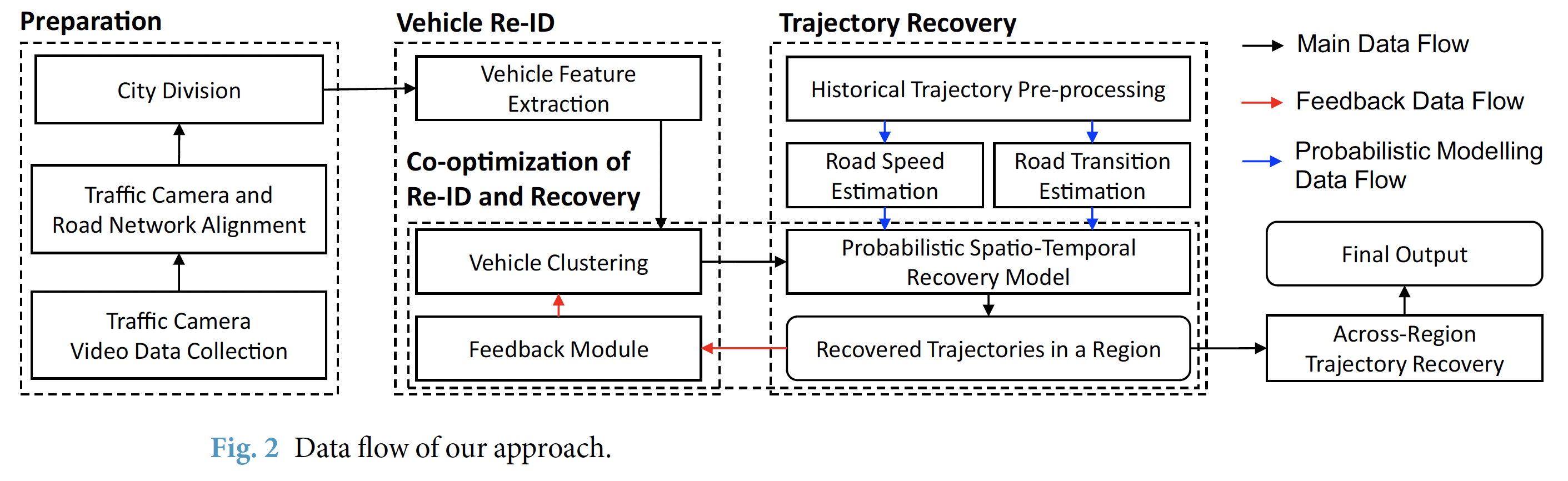
Reference: Yu, Fudan, et al. (2023)
- Preparation 단계
- 데이터를 수집하고, 데이터 처리를 준비하는 단계이다. 본 논문의 저자들은 도로 위 고정식 (단속)카메라에서 수집된 이미지 데이터를 Raw Dataset으로 활용했다고 한다. 이와 동시에, 저자들은 각 도시의 도로 네트워크 데이터를 얻고, 이를 기반으로 Traffic Camera 위치를 맵핑시키는 작업을 수행했다고 한다. 이를 위해 Python OSMnx 패키지를 사용하여 도로망을 구성하고 카메라들의 실제 위치정보를 토대로 가장 가까이 위치한 도로망 노드에 할당시켜 맵핑했다고 한다. 즉 정리하자면, Image Raw Dataset이 도로망의 어떤 Node에서 관찰된 정보인지 대응시키기 위한 것! 이제 카메라에 의해 촬영된 차량 이동 흔적들을 토대로 궤적을 추정하는 그들만의 모델을 적용할 건데, 이에 앞서서 계산에 필요한 Computional Cost를 줄이기 위해 도로망을 조각내는 작업을 선행하여 처리했다고 한다. 여기까지의 흐름이 위 그림에서 기술된 <Traffic Camera Video Data Collection (원천데이터 수집)> - <Traffic Camera and Road Network Alighment (도로네트워크에 카메라위치 맵핑)> - <City Division (도로망 분할)> 작업 수순이다.
- Vehicle Re-ID 단계
- Vehicle Re-Identification 즉, 차량 재식별 단계이다. 특정 한 대의 차량은 도로망을 배회하면서 여러 카메라에 찍혔을텐데, 이 기록들을 식별하여 규합하는 작업이다. 이 단계에서 저자들은 같은 차량인지의 여부를 가리기 위해 ResNet-50 구조의 CNN 모델을 써서 ‘일반적인 차량 외형’과 ‘차량 번호판’에 관한 두 가지의 image feature ($f_a$, $f_p$)로 변환했다. 이 때 얻은 초기 feature들의 차원은 256 by 256인데, 이후 (계산에 용이하게 돌리기 위해) 주성분분석(PCA)을 통해 64 by 64로 차원을 축소하는 작업을 수행했다고 한다. 여기까지 했다고 동일한 차량 기록을 식별할 수 있는 건 아니고, 아직 준비 단계가 더 남았다. 그 다음으로 Trajectory Recovery 단계로 사전준비를 더 진행해야 한다.
- Trajectory Recovery 단계
- 저자들의 논문 속 핵심 모델이라고 할 수 있는 Probability Spatio-Temporal Recovery Model의 파라미터들을 설정하는 단계이다. 문자 그대로, 불연속적인 차량 이동 흔적들을 토대로, 나머지 관측되지 않은 이동 흔적들을 추론하기 위해 나온 모델이다. 기본적으로 관측데이터가 없기 때문에, 경험적으로 ‘어떻게 지나왔을 가능성이 높다’라는 확률적 기대에 의존할 수 밖에 없다. 저자들은 이러한 경험적 확률에 대한 파라미터들을 얻기 위해, Amap이라는 중국 내비게이션 회사의 실제 차량 GPS 이동데이터를 지원받아 계산에 활용했다고 한다.
- Co-optimizaion of Re-ID and Recovery 단계
- 특정 차량에 관해 완전한 궤적을 만들어내는 단계다. Vehicle Feature Extraction 단계에서 얻은 두 개의 features ($f_a$, $f_p$)를 토대로 동일한 차량일 가능성이 높은 기록들끼리 clustering 작업을 수행한다. 이후 Probability Recovery Model을 통과해 동일한 그룹에 속한 기록들을 토대로 나머지 흔적들을 추정하고, 완전한 궤적을 만든다. 이렇게 만들어진 궤적이 특정 가능성의 Threshold 기준치를 만족하지 못하면, 다시 분해되어 clustering 과정으로 진입하고, 이 때 feature $f_a$가 업데이트되어 dynamic feature $f_d$ 파라미터가 새롭게 추가된다. 다시 새롭게 묶인 동일차량 그룹끼리 Probability Recovery Model에 들어가… (반복) … 이 회귀학습과정에서 적절한 궤적이 도출되면 루프를 빠져나온다.
- Across-Region Trajectory Recovery 단계
- 초기 컴퓨팅 계산적 수고를 덜기 위해, 도시를 조각냈다(City Division)고 했다. 사실 이로 인해, 앞서 추정했던 궤적들 역시 퍼즐처럼 조각나있다. 이들을 잘 끼워 맞추는 단계라 보면 된다.
- Final Output
- 이러한 복잡한 절차들을 거쳐서 중국의 두 개 도시(지난시, 선전시)에 대한 차량 궤적 데이터셋이 만들어졌다. 그리고 오늘 살펴볼 데이터가 이것이다. 잘 만들었는지 요리조리 한번 뜯어보자.
1
2
3
4
5
6
7
8
9
10
11
| import os, sys
import pandas as pd, geopandas as gpd, numpy as np
import matplotlib.pyplot as plt
import matplotlib as mpl
import shapely
from shapely.wkt import loads
import datetime as dt
from datetime import datetime
from tqdm import tqdm
import swifter
from collections import defaultdict
|
Road Networks in Jinan and Shenzhen
GeoJSON 파일이면 gpd.read_file(json.dumps(json.load(GeoJSON.json))) 이면 되는데, CSV파일 내 string으로 특별한 규칙(?)으로 LINESTRING 정보를 나열시켜놔서 약간의 전처리가 필요하다.
데이터 컬럼 설명
- edge_jinanOrshenzhen.csv
- Origin, Destination: 시작노드, 종료노드
- Class: 도로종류; Open Street Map(OSM)에서 명시된 도로정보를 참조해 썼다고 한다.
- Geometry: road segment의 Coordinate point(longitude, latitude)가 -로 묶여 있고, LINESTRING 순서가 _를 기준으로 분리되어있다. (WGS84; EPSG-4326)
- Length: road linesting의 meter단위 길이
- node_jinanOrshenzhen.csv
- NodeID: NodeID다.
- Longitude, Latitude: 경도, 위도 (Coordinate point; WGS84)이다.
- HasCamera: 해당 node(intersection)에 고정식 카메라가 있는지의 여부이다. (1: 있음, 0: 없음)
Customized Preprocessing
1
2
3
4
5
6
7
8
9
10
11
12
13
14
15
16
17
18
19
20
21
22
23
24
| # Index 0, 1에 각각 jinan, shenzhen 넣을거임.
network_dataset = [[], []]
# Dataset Loading
for c_idx, city in enumerate(['jinan', 'shenzhen']):
DataPath = os.path.join(os.getcwd(), f'traj_data/{city}')
# 파일명 알파벳 순으로 정렬되기에 edge부터 나오고, 그 다음에 node 데이터 나옴.
for file in os.listdir(DataPath)[:2]:
dataset = pd.read_csv(os.path.join(DataPath, file))
if file.startswith('edge'):
# Geometry에 관한 string타입 데이터 >>> LINESTRING 객체로 전처리 변환
geometry_col = dataset['Geometry'].apply(lambda x: shapely.geometry.LineString(list(map(lambda y: y.split('-'), x.split('_')))))
dataset = dataset.loc[:, dataset.columns!='Geometry']
elif file.startswith('node'):
# 노드(intersection)에 대한 Longitude, Latitude 정보 >>> POINT 객체로 변환
geometry_col = dataset[['Longitude', 'Latitude']].apply(lambda x: shapely.geometry.Point([x[0], x[1]]), axis=1)
else:
raise ValueError("what the hell is this?")
dataset = gpd.GeoDataFrame(dataset, geometry=geometry_col)
network_dataset[c_idx].append(dataset)
|
shenzhen시를 대상으로 어떻게 저장되었는지 확인해보자
1
2
| # shenzhen - edge information
network_dataset[1][0].head()
|
| Origin | Destination | Class | Length | geometry |
|---|
| 0 | 0 | 1 | motorway | 1699.3 | LINESTRING (114.04933 22.69031, 114.04900 22.6... |
|---|
| 1 | 0 | 2 | motorway_link | 663.9 | LINESTRING (114.04933 22.69031, 114.04923 22.6... |
|---|
| 2 | 1 | 10107 | motorway | 152.0 | LINESTRING (114.04845 22.67502, 114.04851 22.6... |
|---|
| 3 | 2 | 8 | motorway_link | 366.4 | LINESTRING (114.04665 22.68507, 114.04619 22.6... |
|---|
| 4 | 2 | 7 | motorway_link | 1202.3 | LINESTRING (114.04665 22.68507, 114.04642 22.6... |
|---|
1
2
| # shenzhen - node information
network_dataset[1][1].head()
|
| NodeID | Longitude | Latitude | HasCamera | geometry |
|---|
| 0 | 0 | 114.049332 | 22.690314 | 0 | POINT (114.04933 22.69031) |
|---|
| 1 | 1 | 114.048449 | 22.675017 | 0 | POINT (114.04845 22.67502) |
|---|
| 2 | 2 | 114.046650 | 22.685071 | 0 | POINT (114.04665 22.68507) |
|---|
| 3 | 3 | 114.048557 | 22.676590 | 0 | POINT (114.04856 22.67659) |
|---|
| 4 | 4 | 114.050360 | 22.681492 | 0 | POINT (114.05036 22.68149) |
|---|
Visualization
1
2
3
4
5
6
7
8
9
10
11
12
13
14
15
16
17
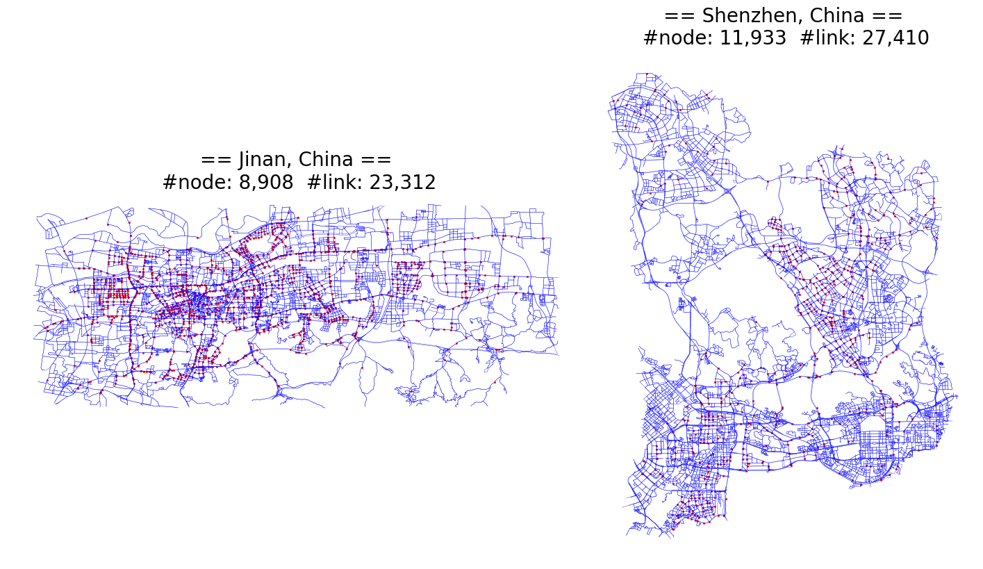
| fig, axs = plt.subplots(nrows=1, ncols=2, facecolor='w', figsize=(18, 10), gridspec_kw={'width_ratios': [1.5, 1]})
for ii, ax in enumerate(axs.flatten()):
# inducing the network size
edge_num, node_num = network_dataset[ii][0].shape[0], network_dataset[ii][1].shape[0]
network_dataset[ii][0].plot(ax=ax, color='blue', linewidth=.25)
node_df = network_dataset[ii][1]
# NOTE THAT!! 카메라가 있는 node intersection만 표시
node_df[node_df.HasCamera==1].plot(ax=ax, color='red', markersize=1.3)
city_name = "Jinan" if ii == 0 else "Shenzhen"
ax.set_title(f"== {city_name}, China ==\n #node: {node_num:,} #link: {edge_num:,}", fontsize=20)
ax.axis('off')
ax.set_aspect('equal')
plt.subplots_adjust(wspace=.01)
plt.show()
|
Trajectory dataset
jinan시는 22년 10월 17일 하루에 대한 차량 궤적 데이터만 존재하고, shenzhen시는 20년 11월 4일, 21년 4월 16일-8월 24일에 대한 차량 궤적 데이터가 존재한다.
데이터 컬럼 설명
- traj_jinanOrshenzhen_date.csv
- VehicleID: 차량 고유식별코드
- TripID: 몇 번째 운행(trip)에 대한 기록인지를 나타내는 인덱스 (동일한 VehicleID, 즉 동일한 하나의 차량은 하루 중 여러 개 운행(trip)기록들이 존재할 수 있다.)
- Points: 운행에 대한 Trajectory가 기록되어 있다. 관측 포인트는 NodeID-Time로 기록되어 있고, 이들은 서로 _(underscore)로 구분되어있다.
- DepatureTime: 운행 기록(첫 관측 포인트)이 시작된 시간이다.
- Duration: DepartureTime부터 운행 기록(마지막 관측 포인트)이 끝난 시간까지 걸린 시간(초 단위)이다.
- Length: Trajectory 동안 운행한 거리(meter 단위)이다.
Important !!! ‘Points’와 ‘DepatureTime’ 컬럼에서의 시간은 하루가 시작되는 시점(00시 00분 00초)에서부터 몇 초가 지난 시점인지로 표기되어 있다.
예를 들어, DepartureTime이 36000.0 이라면, 36000/60/60 = 10:00:00(오전 10시 정각)에 해당 trip의 첫 관측이 이뤄졌다는 의미이다.
Fundamental Profile of dataset
우선 Raw dataset의 DataFrame이 어떻게 생겼는지 직접 확인해보자.
1
2
3
4
5
6
| DataContents = os.listdir(DataPath)
print(DataContents)
* * * * * * * * * * * *
['edge_shenzhen.csv', 'node_shenzhen.csv', 'traj_shenzhen_20210416.csvx', 'traj_shenzhen_20201104.csv', 'traj_shenzhen_20210824.csv']
|
1
2
| traj_dataset = pd.read_csv(os.path.join(DataPath, DataContents[2]))
traj_dataset
|
| VehicleID | TripID | Points | DepartureTime | Duration | Length |
|---|
| 0 | 0 | 0 | 11691-47219.0_982-47314.3_1016-47344.5_1017-47... | 47219.0 | 2412.0 | 10150.1 |
|---|
| 1 | 1 | 0 | 9306-32171.0_11286-32206.7_11287-32224.4_3820-... | 32171.0 | 2291.0 | 7721.5 |
|---|
| 2 | 2 | 0 | 1298-30171.0_4491-30382.7_11723-30397.0_4497-3... | 30171.0 | 1495.0 | 4109.5 |
|---|
| 3 | 2 | 1 | 4180-33688.0_4175-33733.1_4162-33750.4_1236-33... | 33688.0 | 3173.5 | 11457.2 |
|---|
| 4 | 2 | 2 | 6912-39787.0_10508-39871.9_4533-39967.4_4540-4... | 39787.0 | 6035.0 | 32620.8 |
|---|
| ... | ... | ... | ... | ... | ... | ... |
|---|
| 1650248 | 1122380 | 0 | 11928-67501.0_11914-67505.1_8577-67511.2_488-6... | 67501.0 | 21.0 | 7820.5 |
|---|
| 1650249 | 1122381 | 0 | 11776-46358.0_11498-46460.4_11491-47186.3_1148... | 46358.0 | 1861.0 | 655.8 |
|---|
| 1650250 | 1122382 | 0 | 11895-42050.0_11914-42319.5_0-42721.1_1-43564.... | 42050.0 | 4978.0 | 8305.4 |
|---|
| 1650251 | 1122383 | 0 | 8981-34590.0_11576-34937.5_8981-36102.0 | 34590.0 | 1512.0 | 692.4 |
|---|
| 1650252 | 1122384 | 0 | 8981-59141.0_11576-59574.3_8981-60862.0 | 59141.0 | 1721.0 | 692.4 |
|---|
1650253 rows × 6 columns
Remodeling trajectory dataset
- 기존 데이터 구조의 문제점
- DepartureTime 단위는 시점 인식이 쉽지 않고, 데이터 속에서 날짜 식별이 불가능하다.
- ‘Points’ 컬럼에 시간과 궤적 point가 묶여 있어서 분석에 어려움이 있다.
- CSV 포맷의 Data Load 시간이 오래 걸린다.
- 대안
- datetime object (datetime64[ns])로 year, month, date, hour, minute, second 정보를 담는다.
- ‘Points’ 컬럼을 ‘trajectory’컬럼과 ‘ElapseTime’컬럼으로 분리한다.
- pickle(.pkl) 포맷으로 전처리한 데이터를 저장한다.
Note: ‘ElapseTime’컬럼값은 ‘DepartureTime’컬럼 값을 기준으로, 흘러간 시간으로 쓸 생각이다.
1
2
3
4
| # Points 컬럼에서 '궤적에 관한 정보(traj_col)'와 '시점에 관한 정보(timestamp_col)'분리하기.
points_col = traj_dataset['Points'].apply(lambda x: x.split('_'))
traj_col = points_col.apply(lambda x: list(map(lambda y: y.split('-')[0], x))).apply(lambda y: '-'.join(y))
timestamp_col = points_col.apply(lambda x: list(map(lambda y: y.split('-')[1], x)))
|
1
2
3
4
5
6
7
8
9
10
11
12
13
14
15
16
17
| # 궤적에 관한 정보
traj_col
* * * * * * * * * * * *
0 11691-982-1016-1017-7169-7170-7171-214-991-103...
1 9306-11286-11287-3820-1102-1103-1096-11620-109...
2 1298-4491-11723-4497-4538-4540-10259-11739-453...
3 4180-4175-4162-1236-1232-1233-1234-11706-1226-...
4 6912-10508-4533-4540-4538-4497-11723-1298-1285...
...
1650248 11928-11914-8577-488-2777-11574-11575-9343-934...
1650249 11776-11498-11491-11489-11487-11776
1650250 11895-11914-0-1-10107-3903-3904-1468-3673-1092...
1650251 8981-11576-8981
1650252 8981-11576-8981
Name: Points, Length: 1650253, dtype: object
|
1
2
3
4
5
6
7
8
9
10
11
12
13
14
15
16
17
| # 시점에 관한 정보
timestamp_col
* * * * * * * * * * * *
0 [47219.0, 47314.3, 47344.5, 47370.4, 47433.5, ...
1 [32171.0, 32206.7, 32224.4, 32248.1, 32267.6, ...
2 [30171.0, 30382.7, 30397.0, 30530.8, 30603.5, ...
3 [33688.0, 33733.1, 33750.4, 33767.5, 33793.9, ...
4 [39787.0, 39871.9, 39967.4, 40088.6, 40120.9, ...
...
1650248 [67501.0, 67505.1, 67511.2, 67513.1, 67513.6, ...
1650249 [46358.0, 46460.4, 47186.3, 47641.5, 48026.8, ...
1650250 [42050.0, 42319.5, 42721.1, 43564.2, 43656.2, ...
1650251 [34590.0, 34937.5, 36102.0]
1650252 [59141.0, 59574.3, 60862.0]
Name: Points, Length: 1650253, dtype: object
|
raw dataset에서 ‘Duration’ 컬럼 값은 ‘운행이 시작된 시점’과 ‘운행이 끝난 시점’ 사이의 간격이다. 나는 임의의 trip이 어느 시간대(Time window)에 속하는 trip인지 특정하기 위해서 DepartureTime 컬럼 말고도 ArrivalTime 컬럼도 만들려고 했다. 그래서 ‘DepartureTime’컬럼에다가 ‘Duration’컬럼(trip 진행시간)을 더하는 작업을 수행하려다가… 그전에 ‘Points’컬럼에서 뽑아낸 ‘시점에 관한 정보(timestamp_col)’와 ‘Duration’컬럼값이 일치하는지 확인하게 된다.
Note: DepartureTime컬럼값과 trip이 처음 시작된 시점과는 모두 정확히 일치했다.
1
2
3
4
5
6
7
8
9
10
11
12
13
14
15
16
17
18
19
| arrival_time = timestamp_col.apply(lambda x: x[-1]).astype('float64')
departure_time = timestamp_col.apply(lambda x: x[0]).astype('float64')
duration_col = arrival_time - departure_time
# 'Duration'컬럼 값과 Points에서 뽑아낸 Duration 값과의 비교.
diff_duration = duration_col - traj_dataset['Duration']
diff_duration[diff_duration!=0].describe()
* * * * * * * * * * * *
count 4.607200e+04
mean 1.917626e-14
std 2.873179e-12
min -1.159606e-11
25% -2.899014e-12
50% 6.821210e-13
75% 2.899014e-12
max 8.753887e-12
dtype: float64
|
46072개의 trip들에서 아주 근소하지만 Duration 오차가 존재함을 발견했다. 나는 ‘Points’컬럼에서 뽑아낸 ‘시점에 관한 정보(timestamp_col)’를 기준으로 ArrivalTime 컬럼을 만들기로 했다.
1
2
3
4
5
6
7
8
9
10
11
| traj_dataset['ArrivalTime'] = arrival_time
traj_dataset = traj_dataset.drop(columns=['Duration', 'Points'])
traj_dataset['Trajectory'] = traj_col
# ElapseTime 컬럼: 시점에 관한 정보 DepartureTime 기준으로, 흘러간 시간으로 변환해서 기입.
timestamp_col2 = timestamp_col.apply(lambda x: list(map(np.float32, x)))
timestamp_col2 = timestamp_col2.apply(lambda x: list(map(lambda y: round(y, 2), x - x[0])))
timestamp_col2 = timestamp_col2.apply(lambda x: '-'.join(list(map(str, x))))
traj_dataset['ElapseTime'] = timestamp_col2
traj_dataset
|
| VehicleID | TripID | DepartureTime | Length | ArrivalTime | Trajectory | ElapseTime |
|---|
| 0 | 0 | 0 | 47219.0 | 10150.1 | 49631.0 | 11691-982-1016-1017-7169-7170-7171-214-991-103... | 0.0-95.3-125.5-151.4-214.5-241.7-280.4-340.8-4... |
|---|
| 1 | 1 | 0 | 32171.0 | 7721.5 | 34462.0 | 9306-11286-11287-3820-1102-1103-1096-11620-109... | 0.0-35.7-53.4-77.1-96.6-120.9-147.5-169.7-196.... |
|---|
| 2 | 2 | 0 | 30171.0 | 4109.5 | 31666.0 | 1298-4491-11723-4497-4538-4540-10259-11739-453... | 0.0-211.7-226.0-359.8-432.5-569.7-887.3-929.6-... |
|---|
| 3 | 2 | 1 | 33688.0 | 11457.2 | 36861.5 | 4180-4175-4162-1236-1232-1233-1234-11706-1226-... | 0.0-45.1-62.4-79.5-105.9-115.9-139.0-190.4-196... |
|---|
| 4 | 2 | 2 | 39787.0 | 32620.8 | 45822.0 | 6912-10508-4533-4540-4538-4497-11723-1298-1285... | 0.0-84.9-180.4-301.6-333.9-356.9-407.0-495.5-6... |
|---|
| ... | ... | ... | ... | ... | ... | ... | ... |
|---|
| 1650248 | 1122380 | 0 | 67501.0 | 7820.5 | 67522.0 | 11928-11914-8577-488-2777-11574-11575-9343-934... | 0.0-4.1-10.2-12.1-12.6-13.1-13.7-14.9-15.5-15.... |
|---|
| 1650249 | 1122381 | 0 | 46358.0 | 655.8 | 48219.0 | 11776-11498-11491-11489-11487-11776 | 0.0-102.4-828.3-1283.5-1668.8-1861.0 |
|---|
| 1650250 | 1122382 | 0 | 42050.0 | 8305.4 | 47028.0 | 11895-11914-0-1-10107-3903-3904-1468-3673-1092... | 0.0-269.5-671.1-1514.2-1606.2-2114.5-2666.8-27... |
|---|
| 1650251 | 1122383 | 0 | 34590.0 | 692.4 | 36102.0 | 8981-11576-8981 | 0.0-347.5-1512.0 |
|---|
| 1650252 | 1122384 | 0 | 59141.0 | 692.4 | 60862.0 | 8981-11576-8981 | 0.0-433.3-1721.0 |
|---|
1650253 rows × 7 columns
1
2
3
4
5
6
7
8
9
| def Sec2Datetime(ymd, SecTime):
if SecTime >= 86400:
# 하루가 넘어가면
return np.nan
year, month, date = ymd[:4], ymd[4:6], ymd[6:]
MinTime, second = map(int, divmod(SecTime, 60))
hour, minute = divmod(MinTime, 60)
timeObj = datetime.strptime(f'{year}-{month}-{date} {hour:02d}:{minute:02d}:{second:02d}', '%Y-%m-%d %H:%M:%S')
return timeObj
|
1
2
3
4
5
6
| departure_col = traj_dataset['DepartureTime'].apply(lambda x: Sec2Datetime('20210416', x))
arrival_col = traj_dataset['ArrivalTime'].apply(lambda x: Sec2Datetime('20210416', x))
traj_dataset['DepartureTime'] = departure_col
traj_dataset['ArrivalTime'] = arrival_col
traj_dataset
|
| VehicleID | TripID | DepartureTime | Length | ArrivalTime | Trajectory | ElapseTime |
|---|
| 0 | 0 | 0 | 2021-04-16 13:06:59 | 10150.1 | 2021-04-16 13:47:11 | 11691-982-1016-1017-7169-7170-7171-214-991-103... | 0.0-95.3-125.5-151.4-214.5-241.7-280.4-340.8-4... |
|---|
| 1 | 1 | 0 | 2021-04-16 08:56:11 | 7721.5 | 2021-04-16 09:34:22 | 9306-11286-11287-3820-1102-1103-1096-11620-109... | 0.0-35.7-53.4-77.1-96.6-120.9-147.5-169.7-196.... |
|---|
| 2 | 2 | 0 | 2021-04-16 08:22:51 | 4109.5 | 2021-04-16 08:47:46 | 1298-4491-11723-4497-4538-4540-10259-11739-453... | 0.0-211.7-226.0-359.8-432.5-569.7-887.3-929.6-... |
|---|
| 3 | 2 | 1 | 2021-04-16 09:21:28 | 11457.2 | 2021-04-16 10:14:21 | 4180-4175-4162-1236-1232-1233-1234-11706-1226-... | 0.0-45.1-62.4-79.5-105.9-115.9-139.0-190.4-196... |
|---|
| 4 | 2 | 2 | 2021-04-16 11:03:07 | 32620.8 | 2021-04-16 12:43:42 | 6912-10508-4533-4540-4538-4497-11723-1298-1285... | 0.0-84.9-180.4-301.6-333.9-356.9-407.0-495.5-6... |
|---|
| ... | ... | ... | ... | ... | ... | ... | ... |
|---|
| 1650248 | 1122380 | 0 | 2021-04-16 18:45:01 | 7820.5 | 2021-04-16 18:45:22 | 11928-11914-8577-488-2777-11574-11575-9343-934... | 0.0-4.1-10.2-12.1-12.6-13.1-13.7-14.9-15.5-15.... |
|---|
| 1650249 | 1122381 | 0 | 2021-04-16 12:52:38 | 655.8 | 2021-04-16 13:23:39 | 11776-11498-11491-11489-11487-11776 | 0.0-102.4-828.3-1283.5-1668.8-1861.0 |
|---|
| 1650250 | 1122382 | 0 | 2021-04-16 11:40:50 | 8305.4 | 2021-04-16 13:03:48 | 11895-11914-0-1-10107-3903-3904-1468-3673-1092... | 0.0-269.5-671.1-1514.2-1606.2-2114.5-2666.8-27... |
|---|
| 1650251 | 1122383 | 0 | 2021-04-16 09:36:30 | 692.4 | 2021-04-16 10:01:42 | 8981-11576-8981 | 0.0-347.5-1512.0 |
|---|
| 1650252 | 1122384 | 0 | 2021-04-16 16:25:41 | 692.4 | 2021-04-16 16:54:22 | 8981-11576-8981 | 0.0-433.3-1721.0 |
|---|
1650253 rows × 7 columns
1
2
3
4
5
6
7
8
9
10
11
12
13
14
15
16
17
18
| traj_dataset.info()
* * * * * * * * * * * *
<class 'pandas.core.frame.DataFrame'>
RangeIndex: 1650253 entries, 0 to 1650252
Data columns (total 7 columns):
# Column Non-Null Count Dtype
--- ------ -------------- -----
0 VehicleID 1650253 non-null int64
1 TripID 1650253 non-null int64
2 DepartureTime 1650253 non-null datetime64[ns]
3 Length 1650253 non-null float64
4 ArrivalTime 1650253 non-null datetime64[ns]
5 Trajectory 1650253 non-null object
6 ElapseTime 1650253 non-null object
dtypes: datetime64[ns](2), float64(1), int64(2), object(2)
memory usage: 88.1+ MB
|
이런 식으로 Jinan, Shenzhen trajectory dataset들을 모두 변환시켜서 pkl 포맷으로 저장하자.
1
2
3
4
5
6
7
8
9
10
11
12
13
14
15
16
17
18
19
20
21
22
23
24
25
26
27
28
29
30
31
32
33
34
| for city_name in ['jinan', 'shenzhen']:
BasePath = os.path.join(os.getcwd(), f'traj_data/{city_name}')
DataContents = [f for f in os.listdir(BasePath) if f'traj_{city_name}' in f]
for traj_file in tqdm(DataContents):
ymd = traj_file.split('.')[0].split('_')[-1]
filename = f"traj_{city_name}_{ymd}.pkl"
traj_rawdata = pd.read_csv(os.path.join(BasePath, traj_file))
# Points 컬럼에서 '궤적에 관한 정보(traj_col)'와 '시점에 관한 정보(timestamp_col)'분리하기.
points_col = traj_rawdata['Points'].apply(lambda x: x.split('_'))
traj_col = points_col.apply(lambda x: list(map(lambda y: y.split('-')[0], x))).apply(lambda y: '-'.join(y))
timestamp_col = points_col.apply(lambda x: list(map(lambda y: y.split('-')[1], x)))
traj_rawdata['Trajectory'] = traj_col
traj_rawdata['ArrivalTime'] = timestamp_col.apply(lambda x: x[-1]).astype('float64')
departure_col = traj_rawdata['DepartureTime'].apply(lambda x: Sec2Datetime(ymd, x))
arrival_col = traj_rawdata['ArrivalTime'].apply(lambda x: Sec2Datetime(ymd, x))
traj_rawdata['DepartureTime'] = departure_col
traj_rawdata['ArrivalTime'] = arrival_col
traj_rawdata = traj_rawdata.dropna().reset_index(drop=True) # Sec2Datetime에서 np.nan 나온거 제외시키기
traj_rawdata = traj_rawdata.drop(columns=['Duration', 'Points'])
# ElapseTime 컬럼: 시점에 관한 정보 DepartureTime 기준으로, 흘러간 시간으로 변환해서 기입.
timestamp_col = timestamp_col.apply(lambda x: list(map(np.float32, x)))
timestamp_col = timestamp_col.apply(lambda x: list(map(lambda y: round(y, 2), x - x[0])))
timestamp_col = timestamp_col.apply(lambda x: '-'.join(list(map(str, x))))
traj_rawdata['ElapseTime'] = timestamp_col
traj_rawdata.to_pickle(os.path.join(BasePath, filename))
* * * * * * * * * * * *
100%|██████████| 1/1 [02:41<00:00, 161.12s/it]
100%|██████████| 3/3 [18:42<00:00, 374.19s/it]
|
Road Speed from trajectory dataset
trajectory dataset을 통해 Road Speed를 estimate 해보자. Road Speed는 꽤 보편적이면서 분석에 활용하기 좋은 데이터다.
Note: 결론부터 미리 말해두자면, 이 작업은 그다지 만족스런 결과를 내놓지 못했다. ㅠ
1
2
3
4
| BasePath = os.path.join(os.getcwd(), 'traj_data/shenzhen')
shenzhen_files = [f for f in os.listdir(BasePath) if '.pkl' in f]
traj_dataset = pd.read_pickle(os.path.join(BasePath, shenzhen_files[2]))
traj_dataset
|
| VehicleID | TripID | DepartureTime | Length | Trajectory | ArrivalTime | ElapseTime |
|---|
| 0 | 0 | 0 | 2021-08-24 09:49:01 | 784.5 | 8069-3825-3819 | 2021-08-24 10:18:22 | 0.0-713.5-1761.0 |
|---|
| 1 | 0 | 1 | 2021-08-24 15:36:47 | 9484.4 | 11338-11335-3832-3819-3830-10219-9989-4196-977... | 2021-08-24 15:54:38 | 0.0-19.3-36.6-68.0-90.4-98.1-103.9-109.4-116.4... |
|---|
| 2 | 0 | 2 | 2021-08-24 16:56:31 | 2676.0 | 8258-8259-8266-9763-11617-9391-6095-6094-9760-... | 2021-08-24 17:13:42 | 0.0-108.3-235.2-359.3-430.8-460.7-582.8-656.1-... |
|---|
| 3 | 0 | 3 | 2021-08-24 18:54:44 | 1045.3 | 11618-4194-9768-4196-9770-11021-11020-11022-3818 | 2021-08-24 19:09:21 | 0.0-76.9-192.4-408.9-501.4-614.1-665.7-778.4-8... |
|---|
| 4 | 1 | 0 | 2021-08-24 14:07:31 | 8529.2 | 11633-1031-7268-7278-8156-7279-11640-8158-3853... | 2021-08-24 14:37:51 | 0.0-53.8-88.9-115.0-124.6-149.0-155.0-262.7-29... |
|---|
| ... | ... | ... | ... | ... | ... | ... | ... |
|---|
| 1687288 | 1104385 | 0 | 2021-08-24 17:09:14 | 936.7 | 11774-4502-11437-11438-11440-4500-11774 | 2021-08-24 17:35:29 | 0.0-177.3-706.7-784.5-1246.3-1539.5-1575.0 |
|---|
| 1687289 | 1104386 | 0 | 2021-08-24 17:18:58 | 936.7 | 11774-4502-11437-11438-11440-4500-11774 | 2021-08-24 17:58:44 | 0.0-268.6-1070.6-1188.4-1888.0-2332.2-2386.0 |
|---|
| 1687290 | 1104387 | 0 | 2021-08-24 17:45:37 | 936.7 | 11774-4502-11437-11438-11440-4500-11774 | 2021-08-24 17:56:26 | 0.0-73.0-291.2-323.3-513.5-634.4-649.0 |
|---|
| 1687291 | 1104388 | 0 | 2021-08-24 17:42:16 | 936.7 | 11774-4502-11437-11438-11440-4500-11774 | 2021-08-24 18:01:36 | 0.0-130.6-520.5-577.8-917.9-1133.8-1160.0 |
|---|
| 1687292 | 1104389 | 0 | 2021-08-24 17:28:12 | 936.7 | 11774-4502-11437-11438-11440-4500-11774 | 2021-08-24 17:45:31 | 0.0-116.9-466.2-517.5-822.2-1015.6-1039.0 |
|---|
1687293 rows × 7 columns
Converting Procedure
하루단위 trajectory dataset에 대해서 10분 단위로 모든 trip들을 scanning해가며 Road Speed들을 계산한다. 10분 단위로 끊어서 볼 때, 어떤 trip들과 운행정보를 대상에 포함시킬 건지 어떤 기준이 필요하다. 나는 이 기준을 1/2차 필터링으로 나눴고, 최종적으로 필터링되고 남은 trajectory 정보들을 기반으로 Road Speed를 산출했다.
1차 필터링
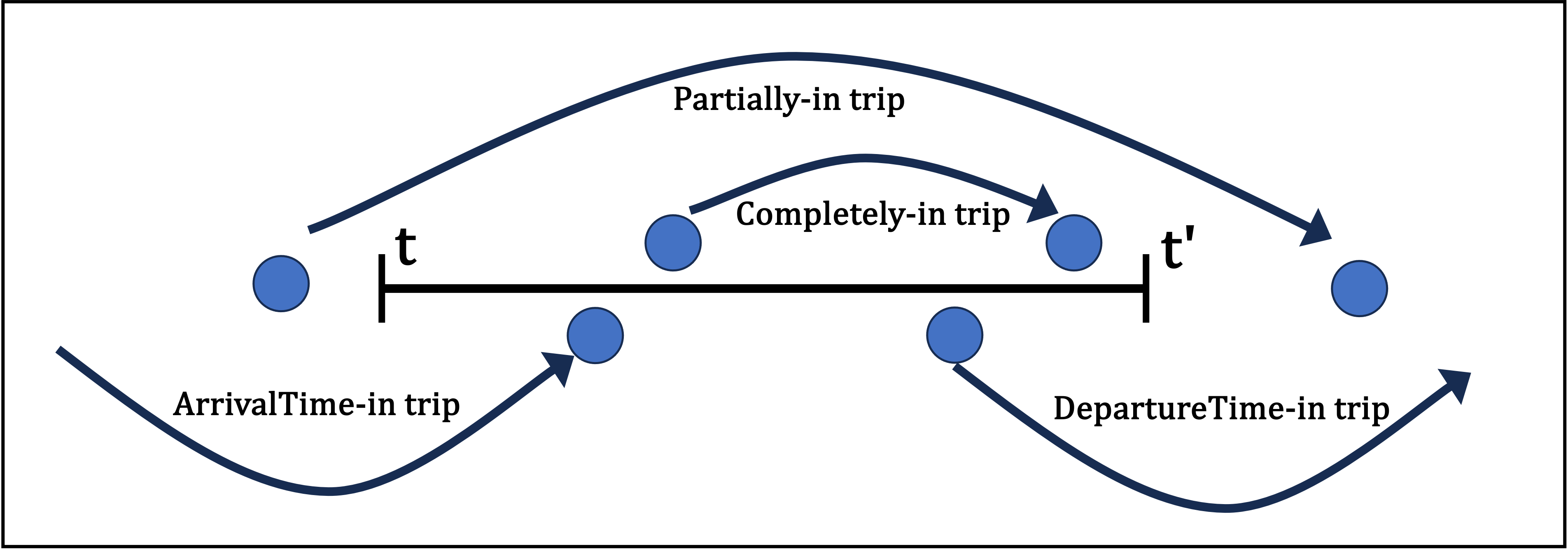
time window를 [t, t’]로 잡고 scanning을 한다고 보면 (나의 경우엔 t’ - t = 10 min),
- t’ < DepatureTime 제외: trip이 나중시간(t’)대비 더 이후에 출발했을 경우 (ex. 7:00~7:10을 보고자 하는데, 7:50에 출발한 trip은 관심대상이 아니다.)
- ArrivalTime < 07:00 제외: trip이 처음시간(t)대비 더 일찍 운행이 종료된 경우 (ex. 7:00~7:10을 보고자 하는데, 6:50에 운행이 끝났던 trip은 관심대상이 아니다.)
즉 1차 필터링 이후, 아래와 같은 trip들만 남게 되는 것이다.
2차 필터링
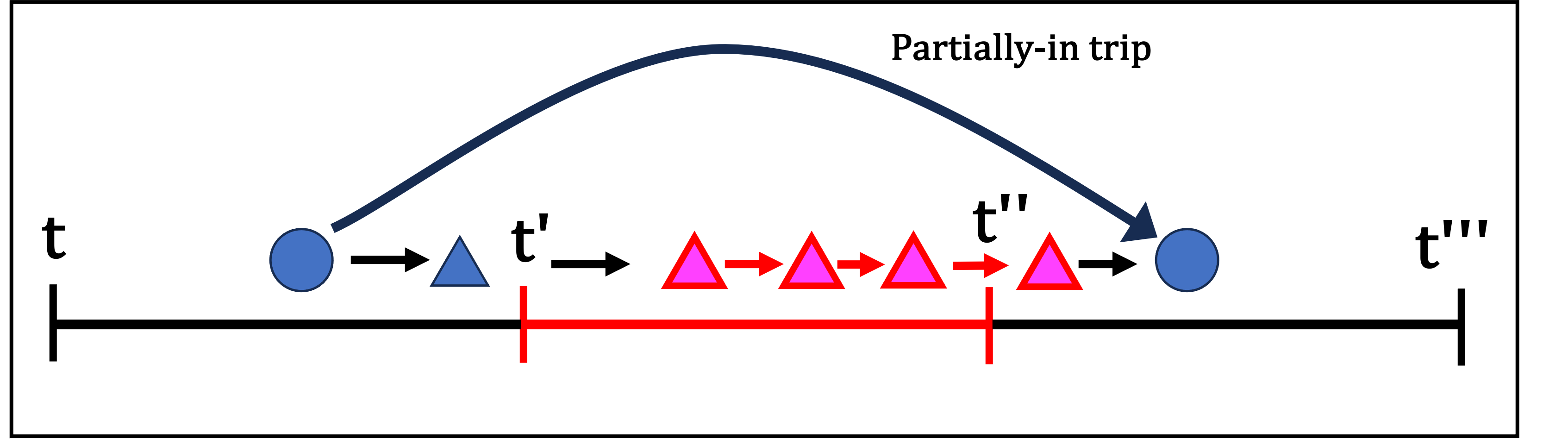
앞서 1차 필터링에서 거르고 남은 trip들을 대상으로 ‘Trajectory’컬럼과 ‘ElapseTime’컬럼 기록들을 하나씩 비교 대조해가며 서칭해야 한다. 그리고 Time Window(10분단위)마다 오버랩되는 부분을 없애기 위해, 또 다른 기준을 세워야 한다. 나는 새로운 Point 기록이 시작된 시점을 기준으로 time window 범위안에 들어오면 관심대상에 넣기로 했다.
다음 그림의 예시처럼, 새로운 Point(Node)가 시작되는 시간을 기준으로 대상에 포함시킨다. (Partially-in, ArrivalTime-in, DepartureTime-in trip 모두 로직은 동일함)
Note 1 : 이게 싫으면 다음 Point(Node)에 도착하는 시간으로 해도 된다. 하지만 둘 중 하나의 기준을 선택해야만, 한 데이터가 두번 쓰이게 되는 중복을 피할 수 있다.
Note 2 : 사실 다시 생각해보면, 본인의 취향과 선택 문제긴 하다. 중복인들 어떠하리. 어차피 두 시간대에 모두 운행한건 맞는데..
Sample Test
로직대로 잘 동작할지 [8:30 ~ 8:40] time window에 관한 필터링을 해보자.
1
2
3
4
5
6
7
8
9
10
| # Test DepartureTime - ArrivalTime 이 08:30~08:40 밖에 있는애들은 완전히 배제
lower_bound_tw = traj_dataset['ArrivalTime'][0].replace(hour=8, minute=30, second=0)
upper_bound_tw = lower_bound_tw.replace(hour=8, minute=40, second=0)
print(lower_bound_tw)
print(upper_bound_tw)
* * * * * * * * * * * *
2021-08-24 08:30:00
2021-08-24 08:40:00
|
1
2
| tw_traj_dataset = traj_dataset.loc[~((traj_dataset['ArrivalTime']<lower_bound_tw) | (traj_dataset['DepartureTime']>upper_bound_tw)), ].reset_index(drop=True)
tw_traj_dataset
|
| VehicleID | TripID | DepartureTime | Length | Trajectory | ArrivalTime | ElapseTime |
|---|
| 0 | 2 | 0 | 2021-08-24 08:21:56 | 22094.2 | 11664-3812-3875-3877-9933-5820-3884-3886-3870-... | 2021-08-24 08:57:45 | 0.0-17.6-53.1-61.0-70.4-99.5-110.0-138.9-145.8... |
|---|
| 1 | 3 | 0 | 2021-08-24 07:30:39 | 439.6 | 11612-11335-4157 | 2021-08-24 08:50:15 | 0.0-566.8-4776.0 |
|---|
| 2 | 13 | 0 | 2021-08-24 08:32:15 | 315.7 | 9306-11286-11614-3822-3822 | 2021-08-24 08:38:41 | 0.0-3.6-5.1-6.0-386.0 |
|---|
| 3 | 17 | 1 | 2021-08-24 08:32:57 | 15407.9 | 11646-3836-3837-9272-3829-3826-11646-3836-3837... | 2021-08-24 09:31:00 | 0.0-17.3-86.7-121.9-134.6-303.9-323.5-338.8-40... |
|---|
| 4 | 19 | 0 | 2021-08-24 07:31:30 | 10480.8 | 11612-11335-4157-8071-8072-4159-4160-3820-1102... | 2021-08-24 08:39:54 | 0.0-28.3-238.1-322.6-478.7-521.6-755.3-968.0-1... |
|---|
| ... | ... | ... | ... | ... | ... | ... | ... |
|---|
| 74196 | 1104036 | 0 | 2021-08-24 08:31:51 | 544.3 | 11898-7079-11931-11898 | 2021-08-24 08:42:23 | 0.0-268.5-589.7-632.0 |
|---|
| 74197 | 1104193 | 0 | 2021-08-24 08:38:26 | 12832.7 | 11901-9994-487-11916-488-2777-11574-2779-2937-... | 2021-08-24 08:51:26 | 0.0-13.3-106.9-122.1-146.1-152.5-157.2-193.2-2... |
|---|
| 74198 | 1104248 | 0 | 2021-08-24 08:34:01 | 357.6 | 1525-6400-1525 | 2021-08-24 08:46:38 | 0.0-353.7-757.0 |
|---|
| 74199 | 1104271 | 0 | 2021-08-24 08:30:50 | 954.9 | 11437-10256-6923-10257-11437 | 2021-08-24 09:21:11 | 0.0-1577.8-1939.2-2530.3-3021.0 |
|---|
| 74200 | 1104296 | 0 | 2021-08-24 08:31:45 | 954.9 | 11437-10256-6923-10257-11437 | 2021-08-24 09:03:39 | 0.0-999.7-1228.6-1603.1-1914.0 |
|---|
74201 rows × 7 columns
1
| tw_traj_dataset.sort_values(by='DepartureTime').head()
|
| VehicleID | TripID | DepartureTime | Length | Trajectory | ArrivalTime | ElapseTime |
|---|
| 17342 | 197077 | 0 | 2021-08-24 06:39:29 | 257.1 | 8258-8268 | 2021-08-24 08:38:22 | 0.0-7133.0 |
|---|
| 1358 | 9961 | 0 | 2021-08-24 06:47:48 | 1260.4 | 11678-867-876-877-1596-11073-11689-10861-7029-... | 2021-08-24 08:43:21 | 0.0-394.1-1049.7-1482.5-2213.6-2774.0-4783.4-5... |
|---|
| 1359 | 9968 | 0 | 2021-08-24 06:48:32 | 6626.8 | 11678-867-868-870-871-11653-873-197-198-2837-2... | 2021-08-24 08:46:44 | 0.0-179.8-400.8-632.8-842.6-921.3-1093.7-1517.... |
|---|
| 1356 | 9958 | 0 | 2021-08-24 06:52:58 | 9555.7 | 11678-867-876-877-11650-1597-884-11652-885-886... | 2021-08-24 08:47:06 | 0.0-118.0-314.4-444.0-575.6-1041.6-1420.0-2201... |
|---|
| 1354 | 9955 | 0 | 2021-08-24 07:00:43 | 8405.9 | 11678-867-868-870-871-11653-873-197-198-2837-2... | 2021-08-24 08:47:29 | 0.0-125.6-292.1-457.4-563.5-617.4-693.4-880.6-... |
|---|
2차 필터링에선 ‘Trajectory’컬럼과 ‘ElapseTime’컬럼을 하나씩 비교 대조해가며 time window안에 들어오는 기록인지 검사한다. 이 과정에서 Link_ID를 추출하고, ElapseTime정보와 도로망 링크길이 정보를 토대로 해당 Link_ID의 속도도 한번에 계산한다.
1
2
3
4
5
6
7
8
9
10
11
12
13
14
15
16
17
18
19
20
21
22
23
24
| def calculate_speed(depTime, traj, elapse):
# 2차 필터링과 속도 계산이 이 함수에서 이루어짐.
nodelist = traj.split('-')
elapseList = list(map(float, elapse.split('-')))
link_list = []
speed_list = []
for i in range(len(nodelist)-1):
if depTime > upper_bound_tw:
break
if depTime < lower_bound_tw:
continue
link = '_'.join(nodelist[i:i+2])
link_df = link_info[link_info['LinkID']==link]
if link_df.empty:
continue
length = link_df['Length'].values[0]
t = np.diff(elapseList[i:i+2])[0]
if t == 0:
continue
spd_kmh = round(length / t * 3.6, 2) # m/s to km/h
speed_list.append(spd_kmh)
link_list.append(link)
depTime = depTime + dt.timedelta(seconds=t)
return link_list, speed_list
|
1
2
3
4
5
| # Shenzhen link information
link_info = network_dataset[1][0]
link_info = pd.concat([pd.DataFrame(link_info.apply(lambda x: '_'.join(map(str, [x.Origin, x.Destination])), axis=1), columns=['LinkID']), link_info['Length']], axis=1)
link_spd = tw_traj_dataset[['DepartureTime', 'Trajectory', 'ElapseTime']].swifter.apply(lambda x: calculate_speed(x[0], x[1], x[2]), axis=1)
|
1
2
3
4
5
| scanning_results = defaultdict(list)
for i in tqdm(range(link_spd.values.shape[0])):
one_trip = list(zip(link_spd[i][0], link_spd[i][1]))
for link_id, spd in one_trip:
scanning_results[link_id].append(spd)
|
1
2
| spd_road_dataset = pd.DataFrame([{'LinkID': link_id, 'RoadSpeed': spd} for link_id, spd in scanning_results.items()])
spd_road_dataset
|
| LinkID | RoadSpeed |
|---|
| 0 | 9306_11286 | [234.7, 704.1, 2816.4, 162.48, 112.66, 68.14, ... |
|---|
| 1 | 11286_11614 | [110.88, 332.64, 831.6, 79.2, 55.44, 33.26, 23... |
|---|
| 2 | 11614_3822 | [139.6, 96.65, 62.82, 39.26, 314.1, 96.65, 11.... |
|---|
| 3 | 11646_3836 | [46.92, 53.06, 62.93, 1159.71, 4059.0, 80.38, ... |
|---|
| 4 | 3836_3837 | [43.38, 48.95, 58.01, 1038.17, 3763.35, 74.34,... |
|---|
| ... | ... | ... |
|---|
| 9352 | 6936_6939 | [2.29] |
|---|
| 9353 | 6550_6547 | [19.31] |
|---|
| 9354 | 6492_6494 | [24.35] |
|---|
| 9355 | 6532_6530 | [26.59] |
|---|
| 9356 | 6530_6531 | [19.91] |
|---|
9357 rows × 2 columns
8:30~8:40 time window 사이에 운행이 관찰된 도로링크 수는 9357개이다. 중국 선전시의 도로링크 수가 27410개를 충분히 커버하진 못한다. 아무래도 trajectory 관찰 장비가 도로위의 카메라에 기반하였고, 이로 인해 모든 도로링크의 동향을 파악할 순 없던 걸로 생각된다.
여기까지 얻어낸 이 데이터 형태를 Road Speed for each road segment에 대한 Raw Dataset로 여기고, 10분 단위 raw dataset을 저장시키기로 한다.
Outlier Detection and Clearing
계산 이후의 DataFrame을 얼핏 보아도 이상치 도로속도가 보인다. 이러한 이상치들은 “직관적 방법”과 “통계적 방법”을 사용해서 걸러내도록 하겠다.
“직관적 방법”은 통상 도로 평균 속도가 몇 시속 km/h 이하로 관찰되야 납득이 되는 속도인지 대한 판단이다. 나는 좀 널럴하게… 도로속도가 120km/h 이상으로 계산된 기록은 제거했다.
“통계적 방법”으로 통상 IQR, Clustering 같은 방법들을 맗한다. 나는 여기서 Median Absolute Deviation(MAD) 방법을 사용했다. Modified z-score (또는 Robust z-score라고도 불리는 듯)로 데이터 값들을 변환하고, 통상 +/- 3.5를 cut-off값으로 쓰는 방법이다. 해당 outlier 탐지 및 제거방식은 아래 1993년 논문에서 처음 제시되었고, 여전히 많이 쓰이는 방법 중 하나이다.
- Iglewicz, Boris, and David C. Hoaglin. “Volume 16: how to detect and handle outliers.” Quality Press, 1993.
1
| np.set_printoptions(suppress=True)
|
1
2
3
4
5
6
7
8
9
10
11
12
13
14
15
16
17
18
19
20
| def OutlierFilter(spd_list, base_spd=120):
if not isinstance(spd_list, np.ndarray):
spd_list = np.array(spd_list)
# Firstly cut-off with base_spd (km/h)
spd_list = spd_list[spd_list<=base_spd]
if len(spd_list) > 1:
# Median Absolute Deviation (MAD) Outlier Detection and Clearing
# Basically its cut-off is (+/-) 3.5.
# Iglewicz, Boris, and David C. Hoaglin. <Volume 16: how to detect and handle outliers.> Quality Press, 1993.
median = np.median(spd_list)
MAD = np.median(abs(spd_list - median))
modified_z_spd = (0.6745 * (spd_list - median)) / MAD
spd_list = spd_list[np.logical_and(modified_z_spd<3.5, modified_z_spd>-3.5)]
if len(spd_list) == 0:
spd_list = np.nan
return spd_list
|
1
2
3
| spd_road_dataset['RoadSpeed'] = spd_road_dataset['RoadSpeed'].apply(lambda x: OutlierFilter(x, base_spd=120))
spd_road_dataset = spd_road_dataset.dropna().reset_index(drop=True)
spd_road_dataset
|
| LinkID | RoadSpeed |
|---|
| 0 | 9306_11286 | [112.66, 68.14, 44.24, 19.29, 37.89, 108.32, 8... |
|---|
| 1 | 11286_11614 | [110.88, 79.2, 55.44, 33.26, 79.2, 118.8, 9.45... |
|---|
| 2 | 11614_3822 | [96.65, 62.82, 39.26, 96.65, 11.12, 62.82, 83.... |
|---|
| 3 | 11646_3836 | [46.92, 53.06, 62.93, 80.38, 91.21, 46.12, 36.... |
|---|
| 4 | 3836_3837 | [43.38, 48.95, 58.01, 74.34, 84.1, 42.64, 33.5... |
|---|
| ... | ... | ... |
|---|
| 8382 | 6936_6939 | [2.29] |
|---|
| 8383 | 6550_6547 | [19.31] |
|---|
| 8384 | 6492_6494 | [24.35] |
|---|
| 8385 | 6532_6530 | [26.59] |
|---|
| 8386 | 6530_6531 | [19.91] |
|---|
8387 rows × 2 columns
도로링크별 속도 기록들에 대해 이상치 작업을 수행했고, 이후 1000여개의 도로링크들은 아예 제거되었다. 이제 이들을 가지고 최종 평균도로속도(RoadSpeed)를 산출한다.
1
2
| spd_road_dataset['AvgSpeed'] = spd_road_dataset['RoadSpeed'].apply(np.mean)
spd_road_dataset
|
| LinkID | RoadSpeed | AvgSpeed |
|---|
| 0 | 9306_11286 | [112.66, 68.14, 44.24, 19.29, 37.89, 108.32, 8... | 47.970050 |
|---|
| 1 | 11286_11614 | [110.88, 79.2, 55.44, 33.26, 79.2, 118.8, 9.45... | 43.357765 |
|---|
| 2 | 11614_3822 | [96.65, 62.82, 39.26, 96.65, 11.12, 62.82, 83.... | 41.027889 |
|---|
| 3 | 11646_3836 | [46.92, 53.06, 62.93, 80.38, 91.21, 46.12, 36.... | 42.250345 |
|---|
| 4 | 3836_3837 | [43.38, 48.95, 58.01, 74.34, 84.1, 42.64, 33.5... | 39.458749 |
|---|
| ... | ... | ... | ... |
|---|
| 8382 | 6936_6939 | [2.29] | 2.290000 |
|---|
| 8383 | 6550_6547 | [19.31] | 19.310000 |
|---|
| 8384 | 6492_6494 | [24.35] | 24.350000 |
|---|
| 8385 | 6532_6530 | [26.59] | 26.590000 |
|---|
| 8386 | 6530_6531 | [19.91] | 19.910000 |
|---|
8387 rows × 3 columns
1
2
3
4
5
6
7
8
9
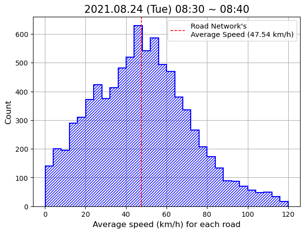
| fig, ax = plt.subplots(facecolor='w', figsize=(7, 5))
spd_road_dataset['AvgSpeed'].hist(ax=ax, color='blue', bins=30, histtype='step', hatch='//////', linewidth=1.5)
roadnet_avgspd = round(spd_road_dataset['AvgSpeed'].mean(), 2)
ax.axvline(roadnet_avgspd, color='red', linewidth=1.1, linestyle='dashed', label=f'Road Network\'s \nAverage Speed ({roadnet_avgspd} km/h)')
ax.set_xlabel("Average speed (km/h) for each road", fontsize=12)
ax.set_ylabel("Count", fontsize=12)
ax.set_title("2021.08.24 (Tue) 08:30 ~ 08:40", fontsize=15)
ax.legend(prop={'size':10.5})
plt.show()
|
1
2
3
4
5
6
7
8
9
10
11
12
13
14
15
16
17
18
19
| target_city = 'shenzhen'
network_label = 0 if target_city == 'jinan' else 1
link_info = network_dataset[network_label][0]
link_info = pd.concat([pd.DataFrame(link_info.apply(lambda x: '_'.join(map(str, [x.Origin, x.Destination])), axis=1), columns=['LinkID']), link_info['Length']], axis=1)
BasePath = os.path.join(os.getcwd(), f'traj_data/{target_city}')
files = [f for f in os.listdir(BasePath) if '.pkl' in f]
print(files)
print()
target_file = files[0]
target_date = target_file.split('.')[0].split('_')[-1]
print(f"For {target_city}, the target date:: {target_date}")
* * * * * * * * * * * *
['traj_shenzhen_20210416.pkl', 'traj_shenzhen_20201104.pkl', 'traj_shenzhen_20210824.pkl']
For shenzhen, the target date:: 20210416
|
1
2
3
4
5
6
7
8
| interval = 10
SavePath = os.path.join(os.getcwd(), f'traj_data/RoadSpeed/{target_city}/{target_date}/{interval}min_interval')
print(SavePath)
target_times = [(h, m) for h in range(7, 20) for m in range(0, 60, interval)] # 07:00 ~ 19:50
* * * * * * * * * * * *
/home/ooooo/VehicleTraj_china/gitlab_share/traj_data/RoadSpeed/shenzhen/20210416/10min_interval
|
1
2
3
4
5
6
7
8
9
10
11
12
13
14
15
16
17
| traj_dataset = pd.read_pickle(os.path.join(BasePath, target_file))
basetime = traj_dataset['ArrivalTime'][0]
for hour, minute in tqdm(target_times[1:]):
lower_bound_tw = basetime.replace(hour=hour, minute=minute, second=0)
upper_bound_tw = lower_bound_tw + dt.timedelta(minutes=interval)
tw_traj_dataset = traj_dataset.loc[~((traj_dataset['ArrivalTime']<lower_bound_tw) | (traj_dataset['DepartureTime']>upper_bound_tw)), ].reset_index(drop=True)
filename = f"roadspeed_{target_city}_{hour:02d}{minute:02d}_{interval}min.pkl"
link_spd = tw_traj_dataset[['DepartureTime', 'Trajectory', 'ElapseTime']].apply(lambda x: calculate_speed(x[0], x[1], x[2]), axis=1)
scanning_results = defaultdict(list)
for i in range(link_spd.values.shape[0]):
one_trip = list(zip(link_spd[i][0], link_spd[i][1]))
for link_id, spd in one_trip:
scanning_results[link_id].append(spd)
spd_road_dataset = pd.DataFrame([{'LinkID': link_id, 'RoadSpeed': spd} for link_id, spd in scanning_results.items()])
spd_road_dataset.to_pickle(os.path.join(SavePath, filename))
|
1
2
3
4
5
6
7
8
9
| target_city = 'shenzhen'
target_date = '20210416'
interval = 10
BasePath = os.path.join(os.getcwd(), f'traj_data/RoadSpeed/{target_city}/{target_date}/{interval}min_interval')
print(BasePath)
* * * * * * * * * * * *
/home/ooooo/VehicleTraj_china/gitlab_share/traj_data/RoadSpeed/shenzhen/20210416/10min_interval
|
1
2
3
4
5
6
7
8
9
10
11
12
13
14
15
16
17
18
19
20
21
22
23
24
25
26
27
28
29
30
| RoadNetAvgSpeed = []
for file in tqdm(os.listdir(BasePath)):
snap_dataset = pd.read_pickle(os.path.join(BasePath, file))
if snap_dataset.empty:
print(f"Empty!!!! {file}")
continue
snap_dataset['RoadSpeed'] = snap_dataset['RoadSpeed'].apply(lambda x: OutlierFilter(x, base_spd=50))
snap_dataset = snap_dataset.dropna().reset_index(drop=True)
snap_dataset['AvgSpeed'] = snap_dataset['RoadSpeed'].apply(np.mean)
road_avg = round(snap_dataset['AvgSpeed'].mean(), 2)
RoadNetAvgSpeed.append(road_avg)
* * * * * * * * * * * *
0%| | 0/78 [00:00<?, ?it/s]
Empty!!!! roadspeed_shenzhen_0700_10min.pkl
Empty!!!! roadspeed_shenzhen_0710_10min.pkl
Empty!!!! roadspeed_shenzhen_0720_10min.pkl
Empty!!!! roadspeed_shenzhen_0730_10min.pkl
Empty!!!! roadspeed_shenzhen_0740_10min.pkl
Empty!!!! roadspeed_shenzhen_0750_10min.pkl
100%|██████████| 78/78 [00:23<00:00, 3.38it/s]
Empty!!!! roadspeed_shenzhen_1900_10min.pkl
Empty!!!! roadspeed_shenzhen_1920_10min.pkl
Empty!!!! roadspeed_shenzhen_1930_10min.pkl
Empty!!!! roadspeed_shenzhen_1940_10min.pkl
Empty!!!! roadspeed_shenzhen_1950_10min.pkl
|
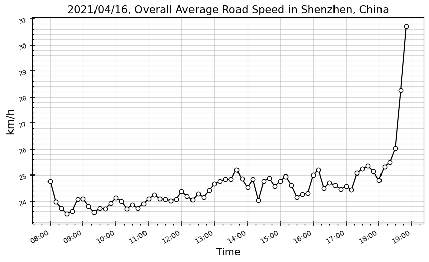
07:00 ~ 19:50 사이 10분 간격으로 도로속도 데이터를 새로 추출했는데, 앞뒤로 1시간 분량이 전처리 과정에서 조건을 만족하지 못하고 전부 제거된 듯하다. 결국 최종적으로 얻은 건 08:00부터 18:50까지의 도로속도 데이터 (Shenzhen 20210416 기준).
Note: 19시 10분 데이터는 있지만, 시각화에서 제외시키기로 한다.
1
2
| time_series = [f'{h:02d}:{m:02d}' for h in range(8, 19) for m in range(0, 60, 10)]
time_xaxis = [datetime.strptime(i, '%H:%M') for i in time_series]
|
1
2
3
4
5
6
7
8
9
10
11
12
13
14
15
16
17
| fig, ax = plt.subplots(facecolor='w', figsize=(10, 6))
ax.plot(time_xaxis, RoadNetAvgSpeed[:-1], marker='o', color='black', markerfacecolor='w')
ax.tick_params(axis='both', which='major', labelsize=10)
ax.tick_params(axis='y', which='major', rotation=15, labelsize=9)
fmt = mpl.dates.DateFormatter('%H:%M')
ax.xaxis.set_major_formatter(fmt)
ax.minorticks_on()
ax.tick_params(which='major', length=7, width=1.2, direction='inout')
ax.tick_params(which='minor', length=2, width=1, direction='in', axis='y')
ax.tick_params(which='minor', length=2.2, width=1, direction='out', axis='x')
ax.grid(which='both', axis='y', alpha=0.5)
ax.grid(which='major', axis='x', alpha=0.5)
ax.set_title("2021/04/16, Overall Average Road Speed in Shenzhen, China", fontsize=15)
ax.set_ylabel("km/h", fontsize=15)
ax.set_xlabel("Time", fontsize=14)
fig.autofmt_xdate()
plt.show()
|
서울시 도로망도 전체 평균도로속도 측면에선 혼잡시간대와 비혼잡시간대의 차이가 그렇게까지 크진 않아서, 정량적인 차이가 크지 않다는 결과는 크게 아쉽진 않다.
다만, 하루 중 흐름의 패턴이 직관과는 다소 반대된다. 아침 출근 시간대에 오히려 원활하고, 점심시간까지 속도가 떨어졌다가, 낮시간부터 서서히 원활해지더니, 저녁 퇴근시간대에 폭발적으로(?) 교통흐름이 원활해진다.
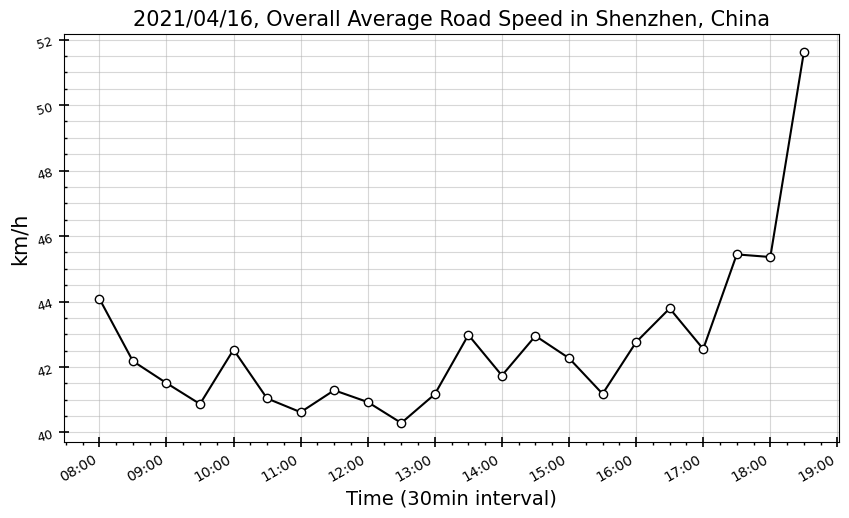
10분 간격의 설정으로 과도하게 resolution을 높힌 탓에, 샘플링수 문제로 부정확한 결과를 발생시켰을 수 있다. 10분 간격 데이터를 3개씩 취합해서, 30분 resolution으로 다시 확인해보자.
1
2
3
4
5
6
7
8
9
10
11
12
13
14
15
16
17
18
19
20
21
22
23
| fileList = os.listdir(BasePath)[6:-6]
RoadNetAvgSpeed = []
for i in tqdm(range(len(fileList)//3)):
binding = fileList[i*3:i*3+3]
binding_dataset = []
for file in binding:
binding_dataset.append(pd.read_pickle(os.path.join(BasePath, file)))
binding_dataset = pd.merge(pd.merge(binding_dataset[0], binding_dataset[1], on='LinkID', how='outer'), binding_dataset[2], on='LinkID', how='outer')
for col in ['RoadSpeed_x', 'RoadSpeed_y', 'RoadSpeed']:
binding_dataset[f"{col}"] = binding_dataset[f"{col}"].apply(lambda x: x if isinstance(x, list) else [])
binding_dataset['RoadSpeed'] = binding_dataset.apply(lambda x: np.concatenate([x['RoadSpeed_x'], x['RoadSpeed_y'], x['RoadSpeed']]), axis=1)
binding_dataset = binding_dataset.iloc[:, [0,3]]
binding_dataset['RoadSpeed'] = binding_dataset['RoadSpeed'].apply(lambda x: OutlierFilter(x, base_spd=120))
binding_dataset = binding_dataset.dropna().reset_index(drop=True)
binding_dataset['AvgSpeed'] = binding_dataset['RoadSpeed'].apply(np.mean)
road_avg = round(binding_dataset['AvgSpeed'].mean(), 2)
RoadNetAvgSpeed.append(road_avg)
* * * * * * * * * * * *
100%|██████████| 22/22 [00:15<00:00, 1.42it/s]
|
1
2
3
4
5
6
7
8
9
10
11
12
13
14
15
16
17
| fig, ax = plt.subplots(facecolor='w', figsize=(10, 6))
ax.plot(time_xaxis[::3], RoadNetAvgSpeed, marker='o', color='black', markerfacecolor='w')
ax.tick_params(axis='both', which='major', labelsize=10)
ax.tick_params(axis='y', which='major', rotation=15, labelsize=9)
fmt = mpl.dates.DateFormatter('%H:%M')
ax.xaxis.set_major_formatter(fmt)
ax.minorticks_on()
ax.tick_params(which='major', length=7, width=1.2, direction='inout')
ax.tick_params(which='minor', length=2, width=1, direction='in', axis='y')
ax.tick_params(which='minor', length=2.2, width=1, direction='out', axis='x')
ax.grid(which='both', axis='y', alpha=0.5)
ax.grid(which='major', axis='x', alpha=0.5)
ax.set_title("2021/04/16, Overall Average Road Speed in Shenzhen, China", fontsize=15)
ax.set_ylabel("km/h", fontsize=15)
ax.set_xlabel("Time (30min interval)", fontsize=14)
fig.autofmt_xdate()
plt.show()
|
패턴은 달라지지 않았다.. 이런 직관과 다른 결과가 나오게 된 가능성은 크게 2가지 정도 생각해볼 수 있겠다.
- 21년 4월 16일(금)에 중국 선전시는 workday가 아니라 어떤 특별한 날일 수 있다.
- Raw 데이터에서 추출한 Trip내 ‘Trajectory’와 ‘ElapseTime’ 정보를 토대로 Length / Time = Velocity 를 계산하는 과정에서 추가적인 이상치 처리가 더 필요할 수 있다.
1번 가능성은 구글링 결과에 의하면 특별한 날처럼 보이진 않는데,,, 아마 2번 가능성처럼 내가 설정한 전처리 과정 외에도 추가적으로 더 세밀한 보정이나 제약을 처리하는 스텝 과정이 필요할 거 같다.
문득, 지금 가지고 있는 다른 (잘 정리된) 도로속도 데이터셋에 대해 소중함을 느끼게 된 시간이다.

 Reference: Yu, Fudan, et al. (2023)