들어가며
이번에 꽤 쓸만한 논문과 데이터를 찾아 냈다. 바로 Kang, Yuhao, et al. (2020). 지난 번, SafeGraph 데이터 포스트에서 언급했던 SafeGraph Inc. 측의 지원을 받아 (행정 단위 스케일이 각기 다른) Multiscale Human Mobility 데이터를 구축한 듯 싶다. 데이터의 전체 양과 그 크기가 상당히 방대하고, 공간 스케일의 granularity 수준이 높다. Scientific Data 저널에 출판된 지 올해로 3년 되었지만, 현재까지 인용수가 151회에 이른다. 그만큼 제각기 연구분석 사례로 활용할 가치가 크다는 의미겠다. 오늘은 이 데이터를 살펴본 내용과 그 과정을 정리해 기록하고자 한다.
Notice for using this dataset
본인의 연구 과제나 논문 등에 타인의 지적 재산을 사용할 때, 인용 문구와 그 출처를 정확히 명시하는 것은 기본 중의 기본임을 잊지 말자.
If you use this dataset in your research or applications, please cite this source:
1
2
3
4
5
6
7
8
9
| @article{kang2020multiscale,
title = {Multiscale Dynamic Human Mobility Flow Dataset in the U.S. during the COVID-19 Epidemic},
author = {Kang, Yuhao and Gao, Song and Liang, Yunlei and Li, Mingxiao and Kruse, Jake},
journal = {Scientific Data},
volumn = {7},
issue = {390},
pages = {1--13},
year = {2020}
}
|
US Human Mobility Dataset during the COVID-19 epidemic
코로나 팬데믹 시기 무렵, 2019년 ~ 2021년 사이, 미국의 유동인구 흐름에 관한 빅데이터.
- 본문 내용에선 2020년 3월 1일 이후부터 당해 연도까지의 데이터만 소개하는데, 출판 이후 저자들은 2019년 1월 1일부터 2021년 12월 사이의 데이터까지 모두 업데이트하였다.
1
2
3
4
5
6
7
8
9
10
11
12
| import os
import pandas as pd
import geopandas as gpd
import numpy as np
import networkx as nx
import matplotlib.pyplot as plt
from collections import defaultdict
from tqdm import tqdm
import requests
import wget
import math
import zipfile
|
Data Structure and Data Acquisition
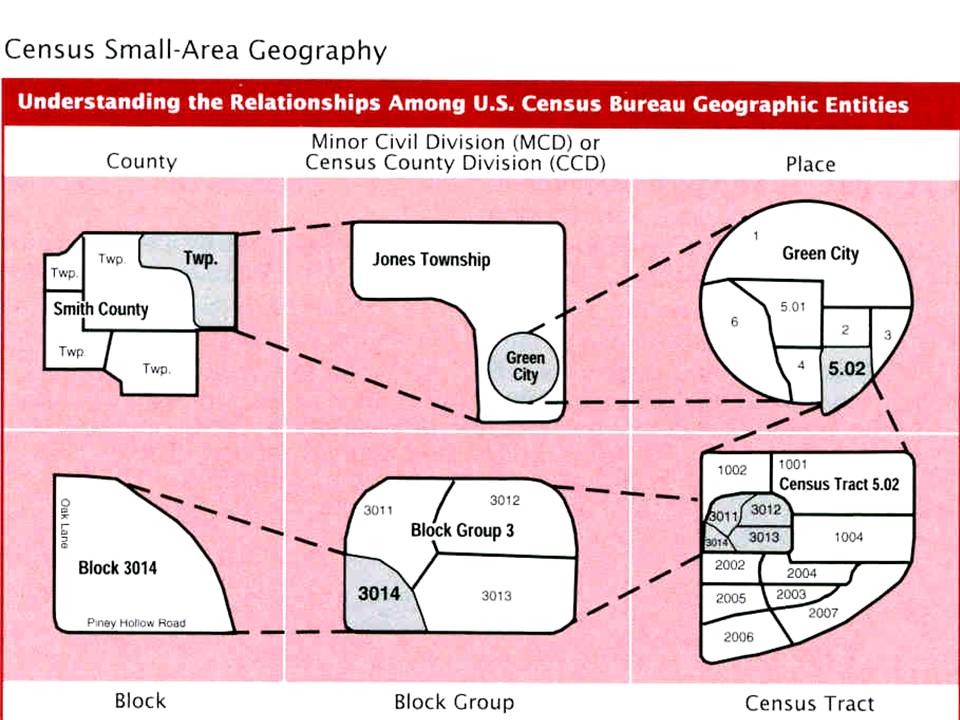
공개 배포 중인 데이터셋은 크게 두 가지 종류이고, 각 종류마다 공간 스케일은 census tract to census tract (ct2ct) / county to county (county2county) / state to state (state2state) 로 나뉜다. 공간 스케일에 대한 이해를 돕기 위해 개념도를 아래 US Census Bureau Geographic Entities 소단원에 첨부해두었다.
- Daily flow dataset: 2019.01.01 ~ 2021.04.15 (ct2ct / county2county / state2state)
- Weekly flow dataset: 2019.01.07 ~ 2021.12.17 (ct2ct / county2county / state2state
추가적인 디테일로는,
- ct2ct 스케일의 데이터는 크기가 너무 커서 20개 파일로 분할되어 있다.
- weekly 데이터의 일자는 해당 주(week)의 월요일 날짜이다.
1
2
3
4
5
6
7
8
9
10
11
12
13
14
15
16
17
18
19
20
21
22
23
24
25
26
27
28
29
30
31
32
33
| US_COVID_MOBILITY
├── daily
│ ├── county2county
│ │ ├── daily_county2county_2019_01_01.csv
│ │ ├── ...
│ │ └── daily_county2county_2021_04_15.csv
│ ├── ct2ct
│ │ └── 2019_01_01
│ │ ├── daily_ct2ct_2019_01_01_0.csv
│ │ ├── ...
│ │ └── daily_ct2ct_2019_01_01_19.csv
│ │ └── ...
│ │ └── 2021_04_15
│ └── state2state
│ ├── daily_state2state_2019_01_01.csv
│ ├── ...
│ └── daily_state2state_2021_04_15.csv
└── weekly
├── county2county
│ ├── weekly_county2county_2019_01_07.csv
│ ├── ...
│ └── weekly_county2county_2021_12_17.csv
├── ct2ct
│ └── 2019_01_07
│ ├── weekly_ct2ct_2019_01_07_0.csv
│ ├── ...
│ └── weekly_ct2ct_2019_01_07_19.csv
│ └── ...
│ └── 2021_12_17
└── state2state
├── weekly_state2state_2019_01_07.csv
├── ...
└── weekly_state2state_2021_12_17.csv
|
1
2
3
4
5
6
7
8
9
10
11
12
13
14
15
16
17
18
19
20
21
22
23
24
25
26
27
28
29
30
31
32
33
34
35
36
37
38
39
40
41
42
43
44
45
46
47
48
49
50
51
52
53
54
55
56
57
58
59
60
61
62
63
64
65
66
67
68
69
70
71
72
73
74
75
76
77
78
79
80
81
82
83
84
85
86
87
88
89
90
91
92
93
94
95
96
97
98
99
100
101
102
103
104
105
106
107
108
109
110
111
112
113
114
115
116
117
118
119
120
121
122
123
124
125
126
127
128
129
130
131
132
133
134
| def download_file(type:str, scale:str, year:str, month:str, day:str, output_folder:str):
"""
Downloads < Daily | Weekly > Flow Dataset for < Kang, Yuhao, et al. 2020 >
Notes that available range
for daily is from 2019.01.01 to 2021.04.15, and
for weekly is from 2019.01.07 to 2021.12.17. (The dataset with country scale may cover the time period starting from 2020.03.02 with the end date being unknown).
Parameters
----------
type : str
daily | weekly
scale : str
ct2ct | county2county | state2state | country2state | country2county | country2ct
Note that the scales of 'country2state | country2county | country2ct' are only available on the 'weekly' type.
Newly note that the scales with 'country' seem to be not available now... Sad... but I've left the country options for opportunities in the future.
year : str
targeting year to download
month : str
targeting month to download (Note that available range for daily is from 2019.01.01 to 2021.04.15)
day : str
targeting day to download (Note that available range for daily is from 2019.01.01 to 2021.04.15)
output_folder : str
BasePath for downloaded file.
Recommend to use 'BasePath' as the path for directories that are divided into 'weekly' and 'daily' by default.
Returns
-------
Boolean
True: Download Succeeded
False: Download Failed
"""
month = month.zfill(2)
day = day.zfill(2)
countryFlag = scale.startswith('country')
try:
if os.path.exists(f"{output_folder}/") == False:
os.mkdir(f"{output_folder}/")
if os.path.exists(f"{output_folder}/{scale}/") == False:
os.mkdir(f"{output_folder}/{scale}/")
except Exception as e:
print(e)
print("There is no output folder. Please create the output folder first!")
if type == 'daily':
try:
if scale == "ct2ct": # ct2ct 스케일에선 하루치 데이터도 워낙 커서 20개로 분할되어 있음. ct2ct 스케일에서는 merging 후처리가 요구됨.
for i in range(20):
if year == "2019":
if (month == "01") or (month == "02") or (month == "03") or (month == "04"):
repo = "DailyFlows-Ct2019-1"
elif (month == "05") or (month == "06") or (month == "07") or (month == "08"):
repo = "DailyFlows-Ct2019-2"
elif (month == "09") or (month == "10") or (month == "11") or (month == "12"):
repo = "DailyFlows-Ct2019-3"
elif year == "2020":
if (month == "01") or (month == "02") or (month == "03") or (month == "04"):
repo = "DailyFlows-Ct2020-1"
elif (month == "05") or (month == "06") or (month == "07") or (month == "08"):
repo = "DailyFlows-Ct2020-2"
elif (month == "09") or (month == "10") or (month == "11") or (month == "12"):
repo = "DailyFlows-Ct2020-3"
elif year == "2021":
repo = "DailyFlows-Ct2021"
r = requests.get(url=f"https://raw.githubusercontent.com/GeoDS/COVID19USFlows-{repo}/master/daily_flows/{scale}/{year}_{month}_{day}/daily_{scale}_{year}_{month}_{day}_{i}.csv")
if r.status_code == 404:
print("404: Not Found. Please check your input parameters of 'scale/year/month/day'.")
return False
else:
if os.path.exists(f"{output_folder}/{scale}/{year}_{month}_{day}/") == False:
os.mkdir(f"{output_folder}/{scale}/{year}_{month}_{day}/")
with open(f"{output_folder}/{scale}/{year}_{month}_{day}/daily_{scale}_{year}_{month}_{day}_{i}.csv", 'wb') as file:
file.write(r.content)
else:
r = requests.get(url=f"https://raw.githubusercontent.com/GeoDS/COVID19USFlows-DailyFlows/master/daily_flows/{scale}/daily_{scale}_{year}_{month}_{day}.csv")
if r.status_code == 404:
print("404: Not Found. Please check your input parameters of 'scale/year/month/day'.")
return False
else:
with open(f"{output_folder}/{scale}/daily_{scale}_{year}_{month}_{day}.csv", 'wb') as file:
file.write(r.content)
return True
except Exception as e:
print(e)
return False
elif type == 'weekly':
try:
if not countryFlag:
if scale == "ct2ct":
for i in range(20):
if year == "2019":
repo = "WeeklyFlows-Ct2019"
elif year == "2020":
repo = "WeeklyFlows-Ct2020"
elif year == "2021":
repo = "WeeklyFlows-Ct2021"
r = requests.get(url=f"https://raw.githubusercontent.com/GeoDS/COVID19USFlows-{repo}/master/weekly_flows/{scale}/{year}_{month}_{day}/weekly_{scale}_{year}_{month}_{day}_{i}.csv")
if r.status_code == 404:
print("404: Not Found. Please check your input parameters of 'scale/year/month/day'.")
return False
else:
if os.path.exists(f"{output_folder}/{scale}/{year}_{month}_{day}/") == False:
os.mkdir(f"{output_folder}/{scale}/{year}_{month}_{day}/")
with open(f"{output_folder}/{scale}/{year}_{month}_{day}/weekly_{scale}_{year}_{month}_{day}_{i}.csv", 'wb') as file:
file.write(r.content)
else:
r = requests.get(url=f"https://raw.githubusercontent.com/GeoDS/COVID19USFlows-WeeklyFlows/master/weekly_flows/{scale}/weekly_{scale}_{year}_{month}_{day}.csv")
if r.status_code == 404:
print("404: Not Found. Please check your input parameters of 'scale/year/month/day'.")
return False
else:
with open(f"{output_folder}/{scale}/weekly_{scale}_{year}_{month}_{day}.csv", 'wb') as file:
file.write(r.content)
return True
else:
r = requests.get(url=f"https://raw.githubusercontent.com/GeoDS/COVID19USFlows/master/weekly_country_flows/{scale}/weekly_{scale}_{year}_{month}_{day}.csv")
if r.status_code == 404:
print("404: Not Found. Please check your input parameters of 'scale/year/month/day'.")
return False
else:
with open(f"{output_folder}/{scale}/weekly_{scale}_{year}_{month}_{day}.csv", 'wb') as file:
file.write(r.content)
return True
except Exception as e:
print(e)
return False
else:
print("Wrong <type> parameter. Choose among 'daily' or 'weekly'.")
return False
|
1
2
3
| # Download a single file
BasePath = './US_COVID_MOBILITY/daily'
download_file('daily', 'state2state', '2019', '1', '3', output_folder=BasePath)
|
결과가 True가 나왔다면, 잘 다운받아졌다는 의미다.
반대로 False가 떠서 실패했다면, 입력한 스케일의 해당 날짜에 데이터가 존재하지 않기 때문에 그런 것이 확률이 제일 크다.
1
2
3
4
5
6
| # Download simultaneously a set of files depicted in a paper of journal.
PaperDates = {'type': ['weekly']*8, \
'scale':['state2state']*4 + ['county2county']*4, \
'year':['2020']*8, 'month':['3','4','5','5']*2, 'day':['2','6','11','25']*2}
PaperDates = pd.DataFrame(PaperDates)
PaperDates
|
| type | scale | year | month | day |
|---|
| 0 | weekly | state2state | 2020 | 3 | 2 |
|---|
| 1 | weekly | state2state | 2020 | 4 | 6 |
|---|
| 2 | weekly | state2state | 2020 | 5 | 11 |
|---|
| 3 | weekly | state2state | 2020 | 5 | 25 |
|---|
| 4 | weekly | county2county | 2020 | 3 | 2 |
|---|
| 5 | weekly | county2county | 2020 | 4 | 6 |
|---|
| 6 | weekly | county2county | 2020 | 5 | 11 |
|---|
| 7 | weekly | county2county | 2020 | 5 | 25 |
|---|
1
2
| BasePath = './US_COVID_MOBILITY/weekly'
PaperDates.apply(lambda x: download_file(x.type, x.scale, x.year, x.month, x.day, output_folder=BasePath), axis=1)
|
1
2
3
4
5
6
7
8
9
| 0 True
1
True
2 True
3 True
4 True
5 True
6 True
7 True
dtype: bool
|
US Census Bureau Geographic Entities
이미지 출처: https://www.census.gov/content/dam/Census/data/developers/geoareaconcepts.pdf
US Geographical Shapefile
배포 중인 데이터셋에는 공간 스케일에 따라 부여되는 GEOID 라는 것이 있다. 이 코드는 US Census Bureau에서 공식적으로 사용하는 식별코드이다. STATE 스케일은 2-자릿수, COUNTY 스케일은 5-자릿수, CENSUS TRACT 스케일은 11-자릿수의 GEOID를 지니고 있다. 추후 Geographic Visualization을 위해 각 스케일에 대한 shapefile이 필요한데, 이 파일은 여기 US Census Bureau 홈페이지에서 찾아볼 수 있다.
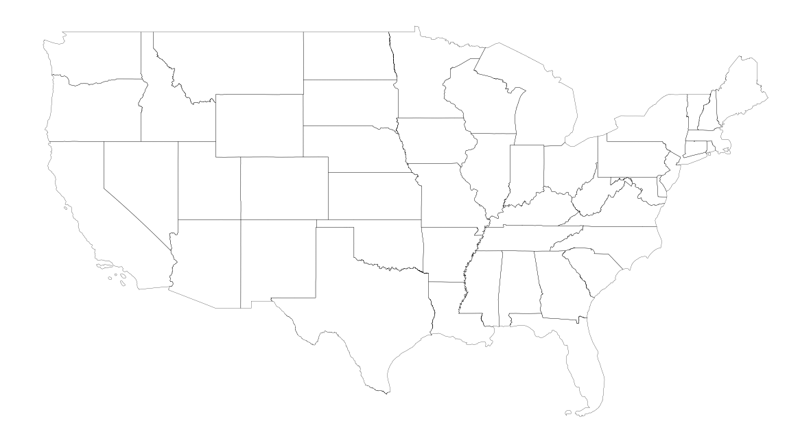
나는 2020년 데이터를 뜯어볼 것이기에 2020년 기준의 shapefile을 내려받아 사용하였다. 그리고 본 글에서는 Contiguous United States (‘하와이주’, ‘알래스카주’를 제외한 Lower 48 States + 워싱턴 D.C) 부분만 살펴보도록 한다.
1
2
3
4
5
6
7
8
9
10
11
12
13
14
15
16
17
| def bar_custom(current, total, width=80):
width=30
avail_dots = width-2
shaded_dots = int(math.floor(float(current) / total * avail_dots))
percent_bar = '[' + '■'*shaded_dots + ' '*(avail_dots-shaded_dots) + ']'
progress = "%d%% %s [%d / %d]" % (current / total * 100, percent_bar, current, total)
return progress
wget.download(url='https://www2.census.gov/geo/tiger/TIGER2020/STATE/tl_2020_us_state.zip', out=os.getcwd(), bar=bar_custom)
wget.download(url='https://www2.census.gov/geo/tiger/TIGER2020/COUNTY/tl_2020_us_county.zip', out=os.getcwd(), bar=bar_custom)
zipList = [zipfile for zipfile in os.listdir() if zipfile.endswith('.zip')]
for file in zipList:
dirName = file.split('.')[0]
if not os.path.exists(f'./{dirName}'):
os.mkdir(f'./{dirName}')
zipfile.ZipFile(os.path.join(os.getcwd(), file)).extractall(f'./{dirName}')
|
1
| 100% [■■■■■■■■■■■■■■■■■■■■■■■■■■■■] [-1 / -1]
|
1
2
| state_shp = gpd.read_file(os.path.join(os.getcwd(), 'tl_2020_us_state'))
county_shp = gpd.read_file(os.path.join(os.getcwd(), 'tl_2020_us_county'))
|
1
2
| state_shp['centroid'] = state_shp.representative_point()
county_shp['centroid'] = county_shp.representative_point()
|
1
2
3
4
5
6
| # Extract 'states' only belonging to the Contiguous United States
state_shp = state_shp[~state_shp['STUSPS'].isin(['PR', 'AK', 'HI', 'AS', 'VI', 'GU', 'MP'])].reset_index(drop=True)
fig, ax = plt.subplots(facecolor='w', figsize=(15, 15))
state_shp.plot(ax=ax, facecolor='None', edgecolor='black', linewidth=0.2)
ax.axis('off')
plt.show()
|
1
2
3
4
5
6
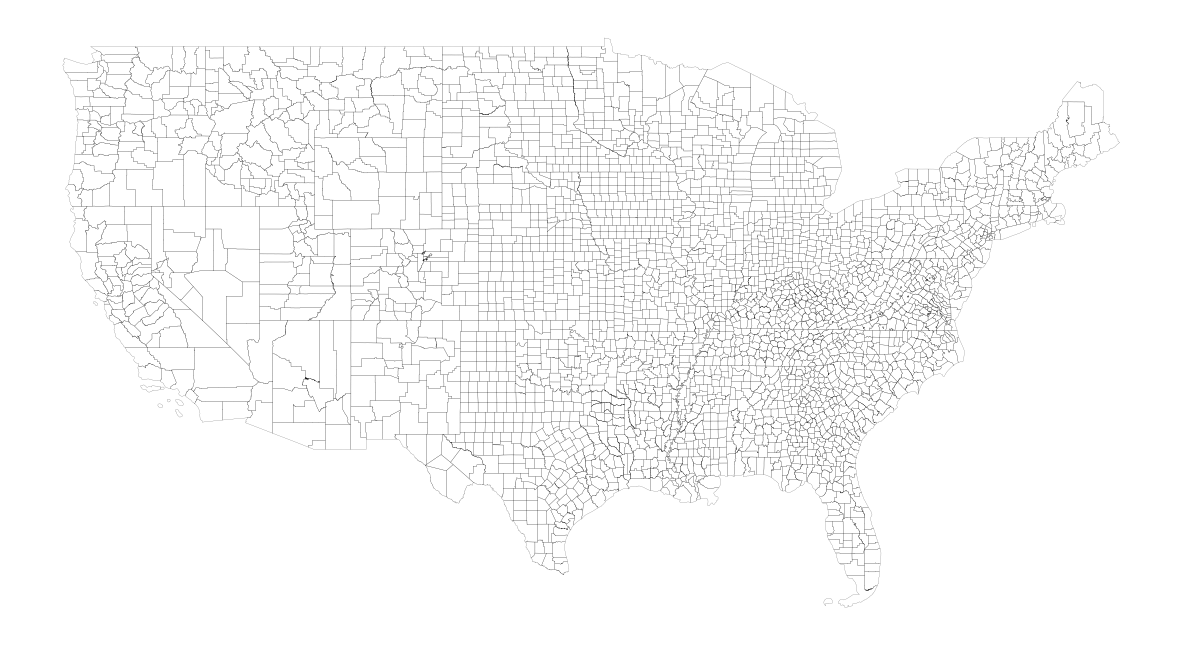
| # Extract 'counties' only belonging to the Contiguous United States
county_shp = county_shp[county_shp['STATEFP'].isin(state_shp['STATEFP'].unique())].reset_index(drop=True)
fig, ax = plt.subplots(facecolor='w', figsize=(15, 15))
county_shp.plot(ax=ax, facecolor='None', edgecolor='black', linewidth=0.1)
ax.axis('off')
plt.show()
|
Daily and Weekly Flow Dataset
Daily Flow와 Weekly Flow 데이터는 모두 OD의 흐름을 보인 Unique한 사람들의 수에 대한 데이터이다. 단지 이를 하루 단위 또는 일주일 단위로 관찰한 것인지에 대한 관찰기간의 차이일 뿐이다.
다시 말해, Weekly Flow에서 특정 OD에 대한 visitor_flows가 100이라면, 일주일 동안 관찰했을 때 해당 OD 흐름을 보인 사람은 Unique하게 딱 100명이라는 말과 동일하다. 즉, 100번의 이동이 있었다라는 의미가 아님 에 유의하자.
여기서 visitor_flows(o, d)는 SafeGraph Inc.가 제공한 모바일 유저들의 궤적-GPS 데이터를 통해 empirical하게 얻어진다. 이후 본 논문에서는 포괄적인 유동인구의 흐름, Dynamical Population Flow을 추론하기 위해, 다음과 같은 공식에 적용한다.
\[pop\_flows(o, d) = visitor\_flows(o, d) \times \frac{pop(o)}{num\_devices(o)}\]
이 때 $pop(o)$는 US Census Bureau에서 수행하는 연간 ACS(American Community Survey)에서 얻어진 $o$란 지역에 거주하는 인구수를 말하고, $num\_devices(o)$는 SafeGraph Inc.의 모바일 데이터 속 고유 고객들 중 $o$ 지역에 거주하는 사람 수를 의미한다. 예를 들어, ACS 조사상 $o$에 거주하는 사람이 1,000명($pop(o)=1000$)이고, SafeGraph 모바일 데이터상 $o$에 거주하는 고객이 100명 존재($num\_devices(o)=100$)하고 이중 30명의 거주민 고객이 $d$로 이동한 것이 관찰($visitor\_flows(o, d)=30$)됐다면, 해당 OD에 대해 추론된 전체 유동 인구적 흐름은 300명($pop\_flows(o, d)=300$)이 되는 것이다.
위의 계산은 모두 기본적으로 CBG(Census Block Group)라는, 본문의 공간 스케일 형태인 Census Tract/ County / State 보다 작은, 스케일에서 계산되었으며 이후 각각의 스케일에 맞게 Aggregation되었다고 한다.
한 가지 유념할 점은, Daily Flow Dataset의 경우 CBG to CBG에 대해 $visitor\_flows(o, d)$를 얻어 적용한 반면에, Weekly Flow Dataset의 경우엔 CBG to POI에 대해 $visitor\_flows(o, d)$를 얻어 위 $pop\_flows$ 계산식에 적용하였다고 한다.
Weekly Flow Dataset
1
2
3
4
5
6
| BasePath = './US_COVID_MOBILITY/weekly'
subdirs = os.listdir(BasePath)
print(subdirs)
state_path = os.path.join(BasePath, subdirs[0])
StateContents = os.listdir(state_path)
print(StateContents)
|
1
2
| ['state2state', 'ct2ct', 'county2county']
['weekly_state2state_2020_03_02.csv', 'weekly_state2state_2020_04_06.csv', 'weekly_state2state_2020_05_11.csv', 'weekly_state2state_2020_05_25.csv']
|
1
2
| week_state_sample = pd.read_csv(os.path.join(state_path, StateContents[0]))
week_state_sample
|
| geoid_o | geoid_d | lng_o | lat_o | lng_d | lat_d | date_range | visitor_flows | pop_flows |
|---|
| 0 | 1 | 1 | -86.844521 | 32.756880 | -86.844521 | 32.756880 | 03/02/20 - 03/08/20 | 3856675 | 38564710.0 |
|---|
| 1 | 1 | 2 | -86.844521 | 32.756880 | -151.250549 | 63.788469 | 03/02/20 - 03/08/20 | 101 | 1009.0 |
|---|
| 2 | 1 | 4 | -86.844521 | 32.756880 | -111.664460 | 34.293095 | 03/02/20 - 03/08/20 | 1652 | 16519.0 |
|---|
| 3 | 1 | 5 | -86.844521 | 32.756880 | -92.439237 | 34.899772 | 03/02/20 - 03/08/20 | 2107 | 21068.0 |
|---|
| 4 | 1 | 6 | -86.844521 | 32.756880 | -119.663846 | 37.215308 | 03/02/20 - 03/08/20 | 3297 | 32968.0 |
|---|
| ... | ... | ... | ... | ... | ... | ... | ... | ... | ... |
|---|
| 2669 | 72 | 51 | -66.414667 | 18.215698 | -78.666349 | 37.510873 | 03/02/20 - 03/08/20 | 358 | 7870.0 |
|---|
| 2670 | 72 | 53 | -66.414667 | 18.215698 | -120.592900 | 47.411639 | 03/02/20 - 03/08/20 | 109 | 2396.0 |
|---|
| 2671 | 72 | 54 | -66.414667 | 18.215698 | -80.613707 | 38.642567 | 03/02/20 - 03/08/20 | 4 | 87.0 |
|---|
| 2672 | 72 | 55 | -66.414667 | 18.215698 | -89.732933 | 44.639944 | 03/02/20 - 03/08/20 | 77 | 1692.0 |
|---|
| 2673 | 72 | 72 | -66.414667 | 18.215698 | -66.414667 | 18.215698 | 03/02/20 - 03/08/20 | 572458 | 12585492.0 |
|---|
2674 rows × 9 columns
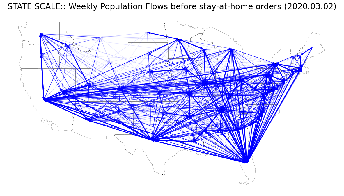
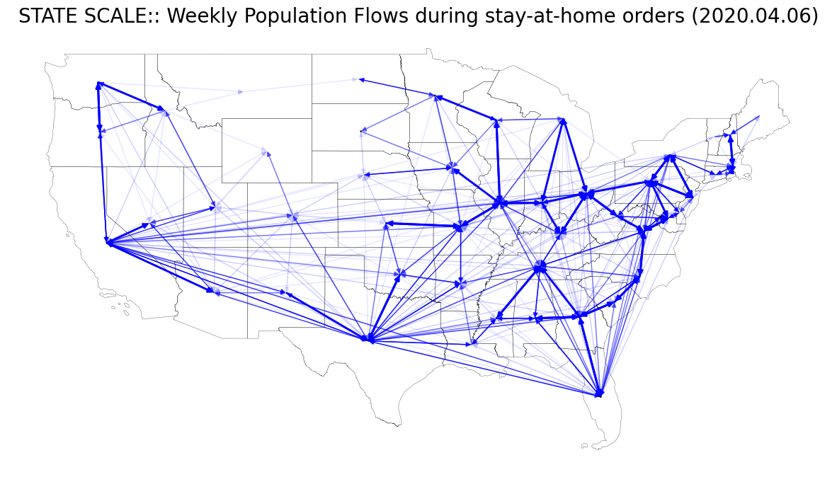
본문의 Fig. 6 (A), (B)를 재현해보자. 이를 위해 총 8개의 weekly flow data를 사용한다.
- Fig. 6 (A)
- weekly_state2state_2020_03_02.csv : before the stay-at-home orders
- weekly_state2state_2020_04_06.csv : during
- weekly_state2state_2020_05_11.csv : after
- weekly_state2state_2020_05_25.csv : after
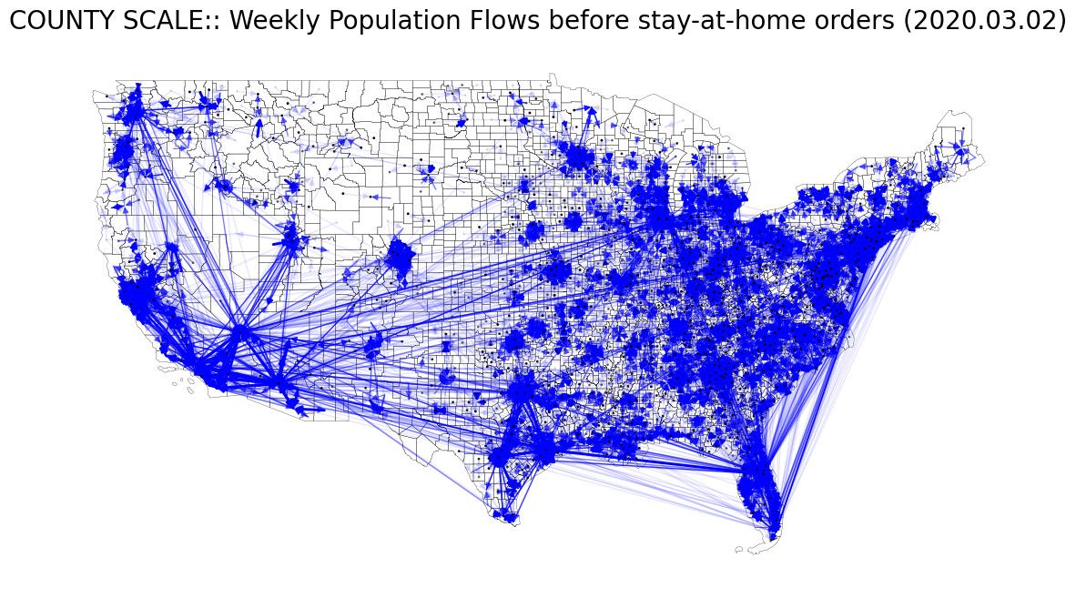
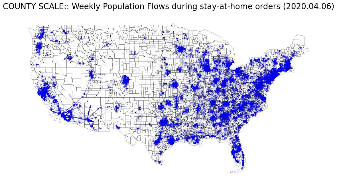
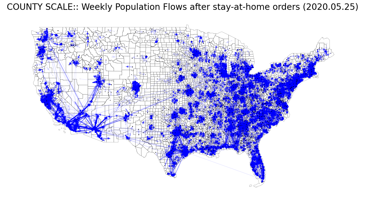
- Fig. 6 (B)
- weekly_county2county_2020_03_02.csv : before
- weekly_county2county_2020_04_06.csv : during
- weekly_county2county_2020_05_11.csv : after
- weekly_county2county_2020_05_25.csv : after
Stay-at-home order는 코로나 팬데믹 무렵 바이러스 확산을 저지하기 위해 정부 기관에 의해 조치된 행정 명령이다. 본 글의 샘플로 활용할 데이터 시기는 코로나 때 미국의 행정 조치(stay-at-home order)가 내려진 전/중/후에 대한 시점을 커버하도록 날짜를 선정한 것이다.
1
2
3
4
5
6
7
8
9
10
11
12
13
14
15
16
17
18
19
20
21
22
23
| # Concatenating by scale
BasePath = './US_COVID_MOBILITY/weekly'
subdirs = os.listdir(BasePath)
state_path = os.path.join(BasePath, subdirs[0])
county_path = os.path.join(BasePath, subdirs[2])
## state2state
StateContents = os.listdir(state_path)
week_state_concat = pd.DataFrame()
for file in StateContents:
sample_ = pd.read_csv(os.path.join(state_path, file))
temp_ = sample_.date_range.apply(lambda x: x.split('-')[:3][0].strip().split('/'))
sample_['main_date'] = temp_.apply(lambda x: f"20{x[2]}{x[0]}{x[1]}")
week_state_concat = pd.concat([week_state_concat, sample_], ignore_index=True)
## county2county
CountyContents = os.listdir(county_path)
week_county_concat = pd.DataFrame()
for file in CountyContents:
sample_ = pd.read_csv(os.path.join(county_path, file))
temp_ = sample_.date_range.apply(lambda x: x.split('-')[:3][0].strip().split('/'))
sample_['main_date'] = temp_.apply(lambda x: f"20{x[2]}{x[0]}{x[1]}")
week_county_concat = pd.concat([week_county_concat, sample_], ignore_index=True)
|
1
2
3
4
5
6
| # Reduce the sets of geoid_o / geoid_d into GEOIDs included in contiguous united states.
interested_state_geoid = state_shp.GEOID.unique().astype(int)
week_state_target = week_state_concat[(week_state_concat['geoid_o'].isin(interested_state_geoid)) & (week_state_concat['geoid_d'].isin(interested_state_geoid))].reset_index(drop=True)
interested_county_geoid = county_shp.GEOID.unique().astype(int)
week_county_target = week_county_concat[(week_county_concat['geoid_o'].isin(interested_county_geoid)) & (week_county_concat['geoid_d'].isin(interested_county_geoid))].reset_index(drop=True)
|
1
2
3
4
5
6
7
8
9
10
11
12
13
14
15
16
17
18
19
20
21
22
23
24
25
26
27
28
29
30
31
32
33
| def fig6a_width_and_alpha(G, weight='pop_flows'):
"""
Optimized with the fig.6 (A) with pop_flows(o, d).
Given the instance of networkx(G), this function generates a sets of width and alpha of edges for drawing in future.
Parameters
----------
G : nx.graph
All edges must have their own weights.
Returns
-------
np.ndarray
with a shape of (x, 2) array containing (width, alpha) for each edges.
"""
wa_cond = lambda x: (0, 0) if x <= 2e4 else \
(1, 0.1) if (2e4 < x) and (x <= 5e4) else \
(1, 0.5) if (5e4 < x) and (x <= 1e5) else \
(1, 0.8) if (1e5 < x) and (x <= 2.5e5) else \
(2.1, 1) if x > 2.5e5 else \
False
width_alpha_arr = []
for s, t in G.edges():
wa = wa_cond(G[s][t][0][weight])
if not isinstance(wa, bool):
width_alpha_arr.append(wa)
else:
print(f"OD not meeting the criteria: {s} > {t}.")
width_alpha_arr.append((0, 0))
return np.array(width_alpha_arr)
|
1
2
3
4
5
6
7
| # Representative points as positions of nodes.
## STATE SCALE
node_pos_dict = defaultdict(list)
for _, row in tqdm(state_shp.iterrows()):
coords = row.centroid.xy
lon, lat = coords[0][0], coords[1][0]
node_pos_dict[int(row.GEOID)] = [lon, lat]
|
1
| 49it [00:00, 10351.61it/s]
|
1
2
3
4
5
6
| # STATE SCALE: 2020. 03. 02 (Before stay-at-home orders)
one_state_target = week_state_target[week_state_target['main_date']=='20200302'].reset_index(drop=True)
one_state_target = one_state_target[one_state_target['geoid_o']!=one_state_target['geoid_d']].reset_index(drop=True)
state_g = nx.MultiDiGraph()
state_g.add_weighted_edges_from(zip(one_state_target['geoid_o'], one_state_target['geoid_d'], one_state_target['pop_flows']), weight='pop_flows')
wa_arr = fig6a_width_and_alpha(state_g)
|
1
2
3
4
5
6
7
| fig, ax = plt.subplots(facecolor='w', figsize=(15, 15))
state_shp.plot(ax=ax, facecolor='None', edgecolor='black', linewidth=.2)
nx.draw_networkx(state_g, pos=node_pos_dict, with_labels=False, node_color='None', edge_color='blue', node_size=1, \
width=wa_arr[:, 0], alpha=wa_arr[:, 1], ax=ax)
ax.set_title("STATE SCALE:: Weekly Population Flows before stay-at-home orders (2020.03.02)", fontsize=20)
ax.axis('off')
plt.show()
|
1
2
3
4
5
6
| # STATE SCALE: 2020. 04. 06 (During stay-at-home orders)
one_state_target = week_state_target[week_state_target['main_date']=='20200406'].reset_index(drop=True)
one_state_target = one_state_target[one_state_target['geoid_o']!=one_state_target['geoid_d']].reset_index(drop=True)
state_g = nx.MultiDiGraph()
state_g.add_weighted_edges_from(zip(one_state_target['geoid_o'], one_state_target['geoid_d'], one_state_target['pop_flows']), weight='pop_flows')
wa_arr = fig6a_width_and_alpha(state_g)
|
1
2
3
4
5
6
7
| fig, ax = plt.subplots(facecolor='w', figsize=(15, 15))
state_shp.plot(ax=ax, facecolor='None', edgecolor='black', linewidth=.2)
nx.draw_networkx(state_g, pos=node_pos_dict, with_labels=False, node_color='None', edge_color='blue', node_size=1, \
width=wa_arr[:, 0], alpha=wa_arr[:, 1], ax=ax)
ax.set_title("STATE SCALE:: Weekly Population Flows during stay-at-home orders (2020.04.06)", fontsize=20)
ax.axis('off')
plt.show()
|
1
2
3
4
5
6
7
8
9
10
11
12
13
14
| # STATE SCALE: 2020. 05. 25 (After stay-at-home orders)
one_state_target = week_state_target[week_state_target['main_date']=='20200525'].reset_index(drop=True)
one_state_target = one_state_target[one_state_target['geoid_o']!=one_state_target['geoid_d']].reset_index(drop=True)
state_g = nx.MultiDiGraph()
state_g.add_weighted_edges_from(zip(one_state_target['geoid_o'], one_state_target['geoid_d'], one_state_target['pop_flows']), weight='pop_flows')
wa_arr = fig6a_width_and_alpha(state_g)
fig, ax = plt.subplots(facecolor='w', figsize=(15, 15))
state_shp.plot(ax=ax, facecolor='None', edgecolor='black', linewidth=.2)
nx.draw_networkx(state_g, pos=node_pos_dict, with_labels=False, node_color='None', edge_color='blue', node_size=1, \
width=wa_arr[:, 0], alpha=wa_arr[:, 1], ax=ax)
ax.set_title("STATE SCALE:: Weekly Population Flows after stay-at-home orders (2020.05.25)", fontsize=20)
ax.axis('off')
plt.show()
|
1
2
3
4
5
6
7
8
9
10
11
12
13
14
15
16
17
18
19
20
21
22
23
24
25
26
27
28
29
30
31
32
33
| def fig6b_width_and_alpha(G, weight='pop_flows'):
"""
Optimized with the fig.6 (B) with pop_flows(o, d).
Given the instance of networkx(G), this function generates a sets of width and alpha of edges for drawing in future.
Parameters
----------
G : nx.graph
All edges must have their own weights.
Returns
-------
np.ndarray
with a shape of (x, 2) array containing (width, alpha) for each edges.
"""
wa_cond = lambda x: (0, 0) if x <= 8e3 else \
(1, 0.1) if (8e3 < x) and (x <= 2e4) else \
(1, 0.5) if (2e4 < x) and (x <= 4e4) else \
(1, 0.8) if (4e4 < x) and (x <= 8e4) else \
(2.1, 1) if x > 8e4 else \
False
width_alpha_arr = []
for s, t in G.edges():
wa = wa_cond(G[s][t][0][weight])
if not isinstance(wa, bool):
width_alpha_arr.append(wa)
else:
print(f"OD not meeting the criteria: {s} > {t}.")
width_alpha_arr.append((0, 0))
return np.array(width_alpha_arr)
|
1
2
3
4
5
6
7
| # Representative points as positions of nodes.
## COUNTY SCALE
node_pos_dict = defaultdict(list)
for _, row in tqdm(county_shp.iterrows()):
coords = row.centroid.xy
lon, lat = coords[0][0], coords[1][0]
node_pos_dict[int(row.GEOID)] = [lon, lat]
|
1
| 3108it [00:00, 12991.84it/s]
|
1
2
3
4
5
6
7
8
9
| # COUNTY SCALE: 2020. 03. 02 (Before stay-at-home orders)
one_county_target = week_county_target[week_county_target['main_date']=='20200302'].reset_index(drop=True)
one_county_target = one_county_target[one_county_target['geoid_o']!=one_county_target['geoid_d']].reset_index(drop=True)
# county 스케일에선 edge수가 현격히 많아져서 (~ 58만개), 그림에서 안보이는 부분인 8000 이하인 OD들은 사전에 미리 제거한다.
one_county_target = one_county_target[one_county_target['pop_flows'] > 8000].reset_index(drop=True)
county_g = nx.MultiDiGraph()
county_g.add_weighted_edges_from(zip(one_county_target['geoid_o'], one_county_target['geoid_d'], one_county_target['pop_flows']), weight='pop_flows')
wa_arr = fig6b_width_and_alpha(county_g)
|
1
2
3
4
5
6
7
| fig, ax = plt.subplots(facecolor='w', figsize=(15, 15))
county_shp.plot(ax=ax, facecolor='None', edgecolor='black', linewidth=.2)
nx.draw_networkx(county_g, pos=node_pos_dict, with_labels=False, node_color='None', edge_color='blue', node_size=1, \
width=wa_arr[:, 0], alpha=wa_arr[:, 1], ax=ax)
ax.set_title("COUNTY SCALE:: Weekly Population Flows before stay-at-home orders (2020.03.02)", fontsize=20)
ax.axis('off')
plt.show()
|
1
2
3
4
5
6
7
8
9
10
11
12
13
14
15
| # COUNTY SCALE: 2020. 04. 06 (During stay-at-home orders)
one_county_target = week_county_target[week_county_target['main_date']=='20200406'].reset_index(drop=True)
one_county_target = one_county_target[one_county_target['geoid_o']!=one_county_target['geoid_d']].reset_index(drop=True)
one_county_target = one_county_target[one_county_target['pop_flows'] > 8000].reset_index(drop=True)
county_g = nx.MultiDiGraph()
county_g.add_weighted_edges_from(zip(one_county_target['geoid_o'], one_county_target['geoid_d'], one_county_target['pop_flows']), weight='pop_flows')
wa_arr = fig6b_width_and_alpha(county_g)
fig, ax = plt.subplots(facecolor='w', figsize=(15, 15))
county_shp.plot(ax=ax, facecolor='None', edgecolor='black', linewidth=.2)
nx.draw_networkx(county_g, pos=node_pos_dict, with_labels=False, node_color='None', edge_color='blue', node_size=1, \
width=wa_arr[:, 0], alpha=wa_arr[:, 1], ax=ax)
ax.set_title("COUNTY SCALE:: Weekly Population Flows during stay-at-home orders (2020.04.06)", fontsize=20)
ax.axis('off')
plt.show()
|
1
2
3
4
5
6
7
8
9
10
11
12
13
14
15
| # COUNTY SCALE: 2020. 05. 25 (After stay-at-home orders)
one_county_target = week_county_target[week_county_target['main_date']=='20200525'].reset_index(drop=True)
one_county_target = one_county_target[one_county_target['geoid_o']!=one_county_target['geoid_d']].reset_index(drop=True)
one_county_target = one_county_target[one_county_target['pop_flows'] > 8000].reset_index(drop=True)
county_g = nx.MultiDiGraph()
county_g.add_weighted_edges_from(zip(one_county_target['geoid_o'], one_county_target['geoid_d'], one_county_target['pop_flows']), weight='pop_flows')
wa_arr = fig6b_width_and_alpha(county_g)
fig, ax = plt.subplots(facecolor='w', figsize=(15, 15))
county_shp.plot(ax=ax, facecolor='None', edgecolor='black', linewidth=.2)
nx.draw_networkx(county_g, pos=node_pos_dict, with_labels=False, node_color='None', edge_color='blue', node_size=1, \
width=wa_arr[:, 0], alpha=wa_arr[:, 1], ax=ax)
ax.set_title("COUNTY SCALE:: Weekly Population Flows after stay-at-home orders (2020.05.25)", fontsize=20)
ax.axis('off')
plt.show()
|
Daily Flow Dataset
1
2
3
4
5
6
| BasePath = './US_COVID_MOBILITY/daily'
subdirs = os.listdir(BasePath)
print(subdirs)
daily_state_path = os.path.join(BasePath, subdirs[2])
DailyStateContents = os.listdir(daily_state_path)
print(DailyStateContents)
|
1
2
| ['ct2ct', 'county2county', 'state2state']
['daily_state2state_2019_01_01.csv', 'daily_state2state_2019_01_02.csv', 'daily_state2state_2019_01_03.csv']
|
1
2
3
| # Daily Flow Dataset 도 'date'에 대한 컬럼만 다를 뿐, 나머지는 동일하다. (weekly flow에선 date_range컬럼)
daily_state_sample = pd.read_csv(os.path.join(daily_state_path, DailyStateContents[0]))
daily_state_sample
|
| geoid_o | geoid_d | lng_o | lat_o | lng_d | lat_d | date | visitor_flows | pop_flows |
|---|
| 0 | 1 | 1 | -86.844521 | 32.756880 | -86.844521 | 32.756880 | 2019-01-01 | 682384 | 8036521.0 |
|---|
| 1 | 1 | 2 | -86.844521 | 32.756880 | -151.593422 | 63.742989 | 2019-01-01 | 17 | 200.0 |
|---|
| 2 | 1 | 4 | -86.844521 | 32.756880 | -111.664460 | 34.293095 | 2019-01-01 | 330 | 3886.0 |
|---|
| 3 | 1 | 5 | -86.844521 | 32.756880 | -92.439237 | 34.899772 | 2019-01-01 | 553 | 6512.0 |
|---|
| 4 | 1 | 6 | -86.844521 | 32.756880 | -119.663846 | 37.215308 | 2019-01-01 | 1267 | 14921.0 |
|---|
| ... | ... | ... | ... | ... | ... | ... | ... | ... | ... |
|---|
| 2685 | 72 | 51 | -66.414667 | 18.215698 | -78.666349 | 37.510873 | 2019-01-01 | 121 | 3712.0 |
|---|
| 2686 | 72 | 53 | -66.414667 | 18.215698 | -120.592900 | 47.411639 | 2019-01-01 | 16 | 490.0 |
|---|
| 2687 | 72 | 54 | -66.414667 | 18.215698 | -80.613707 | 38.642567 | 2019-01-01 | 1 | 30.0 |
|---|
| 2688 | 72 | 55 | -66.414667 | 18.215698 | -89.732933 | 44.639944 | 2019-01-01 | 19 | 583.0 |
|---|
| 2689 | 72 | 72 | -66.414667 | 18.215698 | -66.414667 | 18.215698 | 2019-01-01 | 154693 | 4746667.0 |
|---|
2690 rows × 9 columns
Summary
- COVID-19 팬데믹 기간, 2019년 ~ 2021년 사이의 미국 내 Human Mobility에 대한 Scientific Data 논문을 살펴보았다.
- 본 데이터셋은 SafeGraph Inc.의 모바일 GPS궤적 기반의 visitor_flow 양과 US Census Bureau의 ACS 자료에서 얻은 지역 Population 수를 통해 비례 공식을 적용하여 전체적인 Dynamical Population Flow를 추론해낸 데이터이다.
- 이 때의 visitor_flow의 공간 스케일은 CBG(Census Block Group)단위이고, 이후 Upscaling aggregation을 통해 공간 스케일을 다변화했다.
- visitor_flow는 Daily에선 CBG to CBG 스케일이고, Weekly의 경우엔 CBG to POI 스케일이다.
- 데이터셋은 관찰기간에 따라 크게 Daily, Weekly 로 구분된다.
- 데이터셋은 모두 Origin to Destination(OD) 데이터이고, OD의 공간 스케일에 따라 총 3가지로 다시 나뉜다.
- Census Tract to Census Tract(ct2ct) / County to County(county2county) / State to State(state2state)
- 전체 용량이 0.8 TB에 육박할 정도의 빅데이터이다.
- Scientific Data 본문 내용의 Fig.6 (A), (B)를 재현해보았다.
- Fig. 6 (A): STATE SCALE - before stay-at-home orders / during / after
- Fig. 6 (B): COUNTY SCALE - before / during / after
fin