들어가며
오늘 살펴본 오픈 데이터는 WorldPop 그룹에서 배포하는 세계 각국의 Population - 인구수 데이터이다. WorldPop은 영국 사우샘프턴 대학 산하의 연구 그룹으로, 본인들의 다양한 공간 지리 방법론을 자체 개발하여 이를 토대로 여러 demographic 데이터들을 가공/생산/배포하고 있다. 오늘 살펴볼 Population Counts 말고도 사실, 다양한 속성에 관한 데이터들도 존재하는데… 직접 몇 개 살펴본 바로는 Population Counts 데이터가 시계열적 범위나 대상의 범위 측면으로 봤을 때, 상대적으로 가장 심혈을 기울인 데이터인 듯 하다. WorldPop Hub에 들어가보면, 앞서 이야기한 다양한 속성에 관한 여러 데이터 종류들을 볼 수 있고, 직접 바로 내려받는 것도 가능하다.
WorldPop - Population Counts
1
2
3
4
5
6
7
8
9
10
| import os
import numpy as np, pandas as pd
import matplotlib.pyplot as plt
import geopandas as gpd
from osgeo import gdal
import matplotlib as mpl
from mpl_toolkits.axes_grid1.inset_locator import inset_axes
# osgeo.gdal 모듈을 통해 tif를 다루다 보면 종종 aux.xml 확장자의 메타 데이터를 생성해내는 데, 이를 억제하는 환경 설정임.
os.environ['GDAL_PAM_ENABLED'] = 'NO'
|
Overview
WorldPop Hub - Population Counts 데이터들은 모두 각 나라 속 행정 지역별 인구수를 100m by 100m 또는 1km by 1km cell에 맵핑시킨 grid dataset 이다. ( raster data라고도 함 )
이 때 맵핑하는 방식은 Random Forests Machine Learning method를 사용했다고 하는데, 자세한 내용이 궁금하다면 아래 논문을 참조하자.
Stevens, Forrest R., et al. “Disaggregating census data for population mapping using random forests with remotely-sensed and ancillary data.” PloS one 10.2 (2015)
이 방식을 적용하여 맵핑(행정지역 단위의 인구수 -> 그리드 단위의 인구수)을 진행할 때, ‘지리적 특성(고도, 물길, 해안, 지형의 기울기 etc)’들은 모두 맵핑 과정에 포함되어 처리된다. 이 지리적 특성들에 대한 layer들을 covariate이라고 저자들은 표현한다.
Population Counts 관련 데이터셋들은 크게 두 가지 종류로 나뉘는데 바로 Constrained / Unconstrained 이다.
이 두 데이터셋 사이의 차이는, 맵핑 과정에서 building settlements(주거지 및 건물)에 대한 메타 데이터도 고려했는 지 여부의 차이다.
- Unconstrained: 공통적인 Random Forest(RF) Mapping Estimation만 진행하는 방식.
- Constrained: RF Mapping Estimation을 진행하기 전에, building footprint mask로 사람이 없을 만한 곳은 사전에 한번 거르는 방식.
이런 이유로 종류에 따라 장단점(pros and cons) 또한 명확히 나뉘게 되는데,
- Unconstrained은 사람이 살지 않는(uninhabited regions) 곳에 인구를 할당하는 등의 misallocation 문제들이 존재한다는 단점이 있기에, constrained보다는 부정확하다. 하지만, 이 데이터 형태의 장점으로는 전세계 모든 국가에 대해 2000년부터 2020년까지 연단위 데이터를 배포하고 있어서, 넓은 시기를 아울러서 분석해볼 수 있다는 점이다. 즉, Multi-temporal global data란 장점이 존재한다.
- Constrained는, 반대로, 보다 정확한 맵핑이 된 인구 데이터라는 장점이 있다. 하지만 안타깝게도 2020년 한 해에 대한 데이터만 현재 이용할 수 밖에 없다는 단점이 존재한다. 즉, Not multi-temporal data.
Data Structure
다음과 같이 총 8 가지의 Population Counts 데이터셋이 존재한다.
- Constrained
- Individual Countries 2020 (100m resolution)
- Individual Countries 2020 UN adjusted (100m)
- Unconstrained
- Individual Countries 2000 - 2020 (100m and 1km)
- Individual Countries 2000 - 2020 UN adjusted (100m and 1km)
- Global Mosaics 2000 - 2020 (1km)
- Bespoke Methods Dataset
UN adjusted가 붙은 데이터들은 United Nations(UN)에서 공식적으로 조사한 각국의 총 인구수를 반영해서 재조정한 데이터라고 한다. Global Mosaics은 각국의 100m resolution 데이터를 이어붙여 1km 스케일로 확장시킨 Global Population Counts 데이터이다. Bespoke Methods Dataset은 가장 최근에 추가된 듯한데, RF Mapping 방식이 아닌 Bespoke Mapping이란 방식을 개발해서 적용 후 추출한 raster data인 듯 하다. 본 글에선 RF Mapping으로 추정한 데이터셋들만 살펴보기로 한다.
1
2
3
4
5
6
7
8
9
10
11
12
13
14
15
16
17
18
19
20
21
22
23
24
25
26
27
28
| >>> tree --du -h
worldpop_dataset
├── constrained
│ └── 100m
│ ├── adjusted
│ │ └── KOR
│ │ └── [ 10M] kor_ppp_2020_UNadj_constrained.tif
│ └── no_adjusted
│ └── KOR
│ └── [ 12M] kor_ppp_2020_constrained.tif
└── unconstrained
├── 100m
│ ├── adjusted
│ │ └── KOR
│ │ ├── [ 59M] kor_ppp_2000_UNadj.tif
│ │ ├── ...
│ │ └── [ 59M] kor_ppp_2020_UNadj.tif
│ └── no_adjusted
│ └── KOR
│ ├── [ 68M] kor_ppp_2000.tif
│ ├── ...
│ └── [ 69M] kor_ppp_2020.tif
└── 1km
└── global
├── [1.1G] ppp_2000_1km_Aggregated.tif
├── ...
└── [829M] ppp_2020_1km_Aggregated.tif
|
WorldPop 그룹은 거의 모든 대륙 주요 나라들에 대한 데이터를 배포하고 있다. 하지만 본 글에서는 우리에게 친숙한 한국의 adjusted 100m 데이터(un- and constrained)와 글로벌 1km 데이터들만 다뤄보기로 한다.
1
| BasePath = 'worldpop_dataset/'
|
1
2
3
4
5
6
7
8
9
10
11
12
13
14
15
16
17
18
19
20
21
22
23
24
25
| def AboutTif(tif):
'''
Tiff or Tif 데이터를 로드한 gdal object에 대해 기본적인 정보를 보여주는 함수
'''
num_bands = tif.RasterCount
msg = f"※ Number of bands: {num_bands}"
print(msg)
print(''.ljust(len(msg), '-'))
rows, cols = tif.RasterYSize, tif.RasterXSize
msg = f"※ Raster size: {rows} rows x {cols} columns"
print(msg)
print(''.ljust(len(msg), '-'), end='\n\n')
for bandnum in range(1, num_bands+1):
bandmsg = f" For {bandnum} band "
print(f"{bandmsg:+^{len(msg)}}")
band = tif.GetRasterBand(bandnum)
null_val = band.GetNoDataValue()
print(f"Null value: {null_val}") # " 아, 여긴 확실히 없다. "는 곳을 나타내는 값.
minimum, maximum, mean, sd = band.GetStatistics(True, True)
print(f"Mean: {mean:.3f} / SD: {sd:.3f} / min: {minimum:.3f} / max: {maximum:.3f}")
print(''.ljust(len(msg), '+'), end='\n\n' if num_bands!=1 else '\n')
|
Unconstrained 2000 - 2020 with UN adjusted
1
2
3
4
5
6
| DataPath = os.path.join(BasePath, 'unconstrained', '100m', 'adjusted', 'KOR')
DataContents = os.listdir(DataPath)
print(DataContents)
print()
MyFiles = sorted(DataContents, key=lambda x: int(x.split('_')[2]), reverse=True)[::6]
print(MyFiles)
|
1
2
3
| ['kor_ppp_2020_UNadj.tif', 'kor_ppp_2019_UNadj.tif', 'kor_ppp_2018_UNadj.tif', 'kor_ppp_2016_UNadj.tif', 'kor_ppp_2014_UNadj.tif', 'kor_ppp_2017_UNadj.tif', 'kor_ppp_2012_UNadj.tif', 'kor_ppp_2015_UNadj.tif', 'kor_ppp_2013_UNadj.tif', 'kor_ppp_2010_UNadj.tif', 'kor_ppp_2011_UNadj.tif', 'kor_ppp_2008_UNadj.tif', 'kor_ppp_2006_UNadj.tif', 'kor_ppp_2009_UNadj.tif', 'kor_ppp_2004_UNadj.tif', 'kor_ppp_2007_UNadj.tif', 'kor_ppp_2005_UNadj.tif', 'kor_ppp_2002_UNadj.tif', 'kor_ppp_2003_UNadj.tif', 'kor_ppp_2001_UNadj.tif', 'kor_ppp_2000_UNadj.tif']
['kor_ppp_2020_UNadj.tif', 'kor_ppp_2014_UNadj.tif', 'kor_ppp_2008_UNadj.tif', 'kor_ppp_2002_UNadj.tif']
|
1
| one_dataset = gdal.Open(os.path.join(DataPath, MyFiles[0]))
|
1
2
3
4
5
6
7
8
9
| ※ Number of bands: 1
--------------------
※ Raster size: 6601 rows x 7031 columns
---------------------------------------
+++++++++++++ For 1 band ++++++++++++++
Null value: -99999.0
Mean: 2.773 / SD: 11.252 / min: 0.021 / max: 288.933
+++++++++++++++++++++++++++++++++++++++
|
1
2
3
4
| band_data = one_dataset.GetRasterBand(1)
null_val = band_data.GetNoDataValue()
band_arr = band_data.ReadAsArray().flatten()
band_arr = band_arr[band_arr != null_val]
|
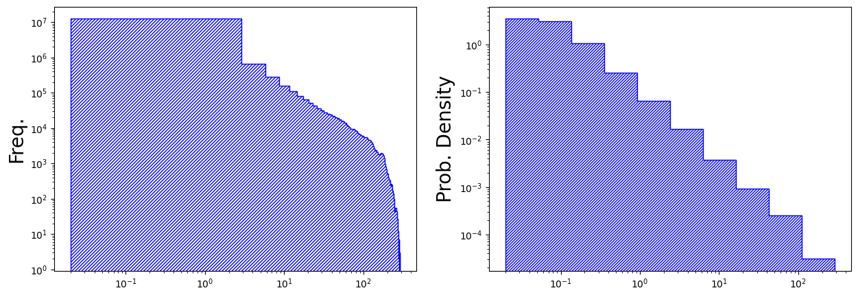
1
2
3
4
5
6
7
8
9
10
11
| fig, axs = plt.subplots(nrows=1, ncols=2, facecolor='w', figsize=(15, 5))
axs[0].hist(band_arr, bins=100, color='blue', histtype='step', hatch='///////')
axs[0].set_ylabel('Freq.', fontsize=20)
axs[0].set_xscale('log')
axs[0].set_yscale('log')
axs[1].hist(band_arr, bins=np.logspace(np.log10(band_arr.min()), np.log10(band_arr.max()), 11), density=True, color='blue', histtype='step', hatch='////////')
axs[1].set_ylabel('Prob. Density', fontsize=20)
axs[1].set_xscale('log')
axs[1].set_yscale('log')
plt.show()
|
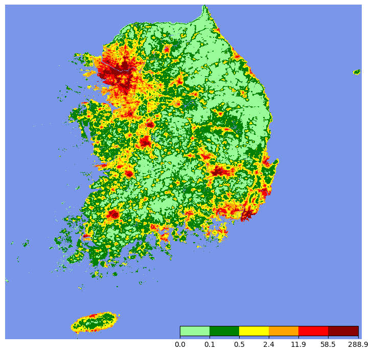
1
2
3
4
5
| cmap = mpl.colors.LinearSegmentedColormap.from_list("", ["palegreen", "green", "yellow", "orange", "red", "darkred"])
logbounds = np.logspace(np.log10(band_arr.min()), np.log10(band_arr.max()), 7)
norm = mpl.colors.BoundaryNorm(logbounds, cmap.N)
cmap.set_under('royalblue', alpha=0.7)
cmap
|
1
2
3
4
5
6
7
8
9
10
| img = band_data.ReadAsArray()
fig, ax = plt.subplots(facecolor='w', figsize=(9, 9))
im = ax.imshow(img, cmap=cmap, norm=norm, interpolation='none')
ax.axis('off')
cb_ax = inset_axes(ax, width="50%", height="3%", loc='lower right')
fig.colorbar(im, cax=cb_ax, orientation='horizontal')
plt.show()
|
1
2
3
4
5
6
7
| # 4개 연도 시각화 비교
for i, file in enumerate(MyFiles[::-1]):
year = file.split('_')[2]
print(f"{year:=^60}")
dataset = gdal.Open(os.path.join(DataPath, file))
AboutTif(dataset)
print(''.ljust(60, '=') if i+1 == len(MyFiles) else '')
|
1
2
3
4
5
6
7
8
9
10
11
12
13
14
15
16
17
18
19
20
21
22
23
24
25
26
27
28
29
30
31
32
33
34
35
36
37
38
39
40
41
42
43
44
| ============================2002============================
※ Number of bands: 1
--------------------
※ Raster size: 6601 rows x 7031 columns
---------------------------------------
+++++++++++++ For 1 band ++++++++++++++
Null value: -99999.0
Mean: 2.285 / SD: 8.758 / min: 0.029 / max: 143.500
+++++++++++++++++++++++++++++++++++++++
============================2008============================
※ Number of bands: 1
--------------------
※ Raster size: 6601 rows x 7031 columns
---------------------------------------
+++++++++++++ For 1 band ++++++++++++++
Null value: -99999.0
Mean: 2.399 / SD: 8.992 / min: 0.028 / max: 144.951
+++++++++++++++++++++++++++++++++++++++
============================2014============================
※ Number of bands: 1
--------------------
※ Raster size: 6601 rows x 7031 columns
---------------------------------------
+++++++++++++ For 1 band ++++++++++++++
Null value: -99999.0
Mean: 2.581 / SD: 10.376 / min: 0.030 / max: 201.992
+++++++++++++++++++++++++++++++++++++++
============================2020============================
※ Number of bands: 1
--------------------
※ Raster size: 6601 rows x 7031 columns
---------------------------------------
+++++++++++++ For 1 band ++++++++++++++
Null value: -99999.0
Mean: 2.773 / SD: 11.252 / min: 0.021 / max: 288.933
+++++++++++++++++++++++++++++++++++++++
============================================================
|
1
2
3
4
5
6
7
8
9
10
11
12
13
14
15
16
17
18
19
20
21
22
23
24
25
26
27
28
29
30
31
32
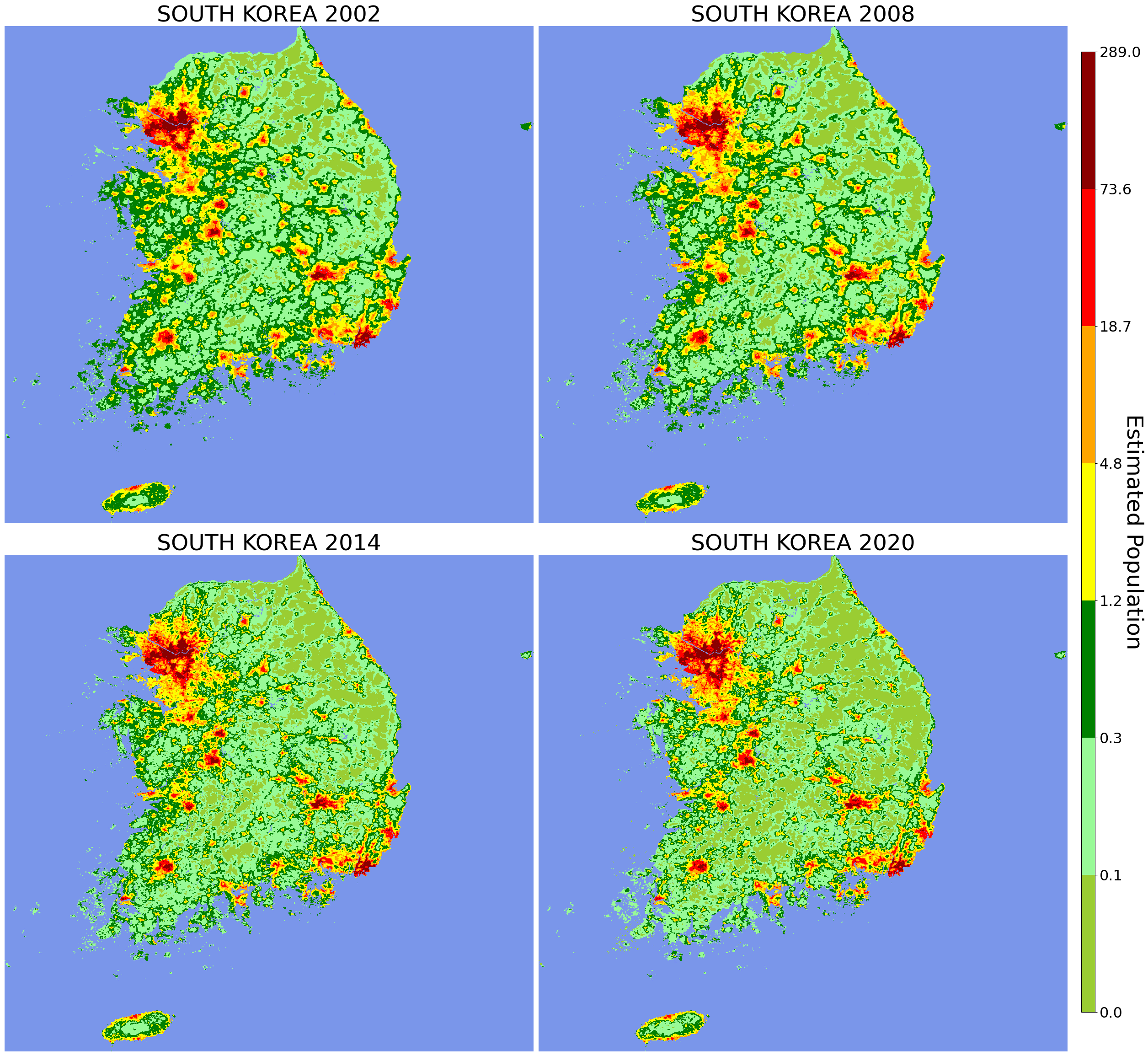
| fig, axs = plt.subplots(nrows=2, ncols=2, facecolor='w', figsize=(30, 30))
cmap = mpl.colors.LinearSegmentedColormap.from_list("", ["yellowgreen", "palegreen", "green", "yellow", "orange", "red", "darkred"])
## Colorbar depending on each value 동일하게 적용
## 전체 관찰 데이터셋의 단일 최소값/최대값으로 Normalization
logbounds = np.logspace(np.log10(0.02), np.log10(289), 8)
norm = mpl.colors.BoundaryNorm(logbounds, cmap.N)
cmap.set_under('royalblue', alpha=0.7)
########################################################
for ax, file in zip(axs.flatten(), MyFiles[::-1]):
year = file.split('_')[2]
dataset = gdal.Open(os.path.join(DataPath, file))
band_data = dataset.GetRasterBand(1)
null_val = band_data.GetNoDataValue()
img = band_data.ReadAsArray()
band_arr = img.flatten()
band_arr = band_arr[band_arr != null_val]
im = ax.imshow(img, cmap=cmap, norm=norm, interpolation='none')
ax.set_title(f"SOUTH KOREA {year}", fontsize=35)
ax.axis('off')
cbar_ax = fig.add_axes([0.91, 0.15, 0.01, 0.7])
cbar = fig.colorbar(im, cax=cbar_ax)
cbar.set_label(label="Estimated Population", size=35, rotation=270)
cbar.ax.tick_params(labelsize=23)
fig.subplots_adjust(hspace=.002, wspace=.01)
plt.show()
|
Comparison between Unconstrained and Constrained
1
2
3
4
5
6
| Tifs = []
for tp in ['unconstrained', 'constrained']:
DataPath = os.path.join(BasePath, tp, '100m', 'adjusted', 'KOR')
for file in os.listdir(DataPath):
if '2020' in file:
Tifs.append(gdal.Open(os.path.join(DataPath, file)))
|
1
2
3
4
| for i, prefix in enumerate(['Unconstrained KOR 2020', 'Constrained KOR 2020']):
print(f"{prefix:=^60}")
AboutTif(Tifs[i])
print(''.ljust(60, '=') if i+1 == 2 else '')
|
1
2
3
4
5
6
7
8
9
10
11
12
13
14
15
16
17
18
19
20
21
22
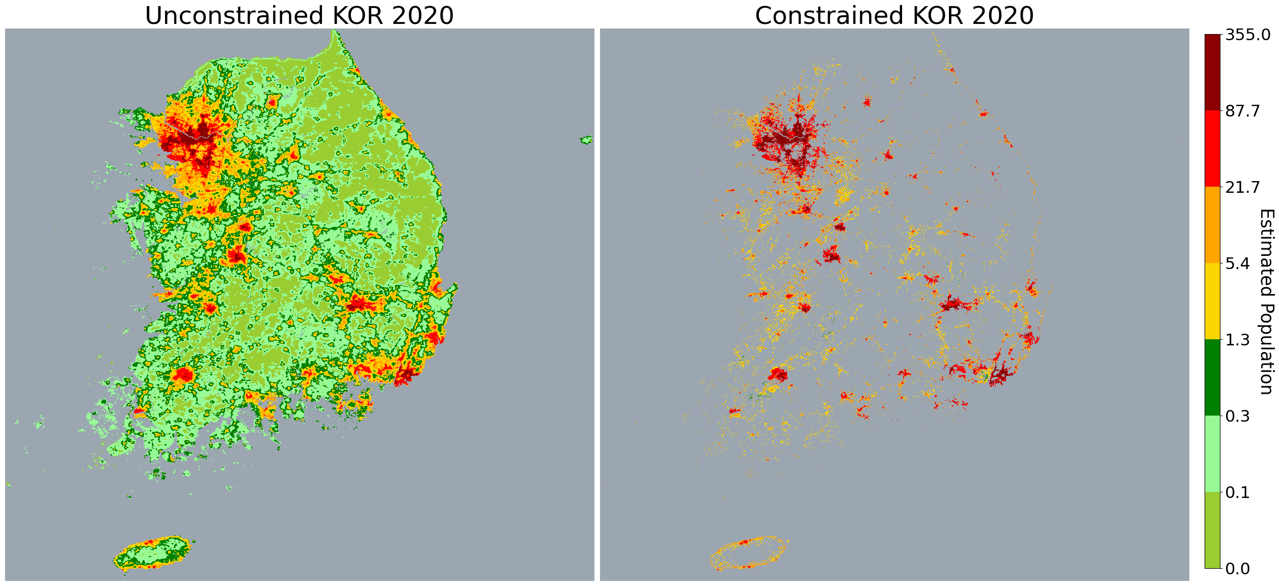
| ===================Unconstrained KOR 2020===================
※ Number of bands: 1
--------------------
※ Raster size: 6601 rows x 7031 columns
---------------------------------------
+++++++++++++ For 1 band ++++++++++++++
Null value: -99999.0
Mean: 2.773 / SD: 11.252 / min: 0.021 / max: 288.933
+++++++++++++++++++++++++++++++++++++++
====================Constrained KOR 2020====================
※ Number of bands: 1
--------------------
※ Raster size: 6601 rows x 7031 columns
---------------------------------------
+++++++++++++ For 1 band ++++++++++++++
Null value: -99999.0
Mean: 29.367 / SD: 41.884 / min: 0.796 / max: 354.886
+++++++++++++++++++++++++++++++++++++++
============================================================
|
1
2
3
4
5
6
7
8
9
10
11
12
13
14
15
16
17
18
19
20
21
22
23
24
25
26
27
28
29
| labelList = ['Unconstrained KOR 2020', 'Constrained KOR 2020']
fig, axs = plt.subplots(nrows=1, ncols=2, facecolor='w', figsize=(30, 15))
cmap = mpl.colors.LinearSegmentedColormap.from_list("", ["yellowgreen", "palegreen", "green", "gold", "orange", "red", "darkred"])
logbounds = np.logspace(np.log10(0.02), np.log10(355), 8)
norm = mpl.colors.BoundaryNorm(logbounds, cmap.N)
cmap.set_under('slategrey', alpha=0.7)
for i, (ax, lb) in enumerate(zip(axs.flatten(), labelList)):
dataset = Tifs[i]
band_data = dataset.GetRasterBand(1)
null_val = band_data.GetNoDataValue()
img = band_data.ReadAsArray()
band_arr = img.flatten()
band_arr = band_arr[band_arr != null_val]
im = ax.imshow(img, cmap=cmap, norm=norm, interpolation='none')
ax.set_title(f"{lb}", fontsize=35)
ax.axis('off')
cbar_ax = fig.add_axes([0.91, 0.15, 0.01, 0.7])
cbar = fig.colorbar(im, cax=cbar_ax)
cbar.set_label(label="Estimated Population", size=25, rotation=270)
cbar.ax.tick_params(labelsize=23)
fig.subplots_adjust(wspace=.01)
plt.show()
|
1
2
3
4
5
6
7
8
| def CountNull(band):
nullval = band.GetNoDataValue()
img_arr = band.ReadAsArray().flatten()
nullcnt = sum(img_arr == null_val)
return nullcnt
uncon_nullcnt = CountNull(Tifs[0].GetRasterBand(1))
con_nullcnt = CountNull(Tifs[1].GetRasterBand(1))
|
1
2
3
4
5
6
7
8
| totSize = Tifs[0].RasterXSize * Tifs[0].RasterYSize
msg = f"KOR 래스터 데이터 내 Grid 갯수: {totSize:,} Grids"
print(msg)
print(''.ljust(len(msg), '-'))
print("확실히 사람이 없는 곳이라고 판단하는 그리드 갯수가")
print(f"※ Unconstrained KOR 2020 : {uncon_nullcnt:,} 개")
print(f"※ Constrained KOR 2020 : {con_nullcnt:,} 개")
|
1
2
3
4
5
| KOR 래스터 데이터 내 Grid 갯수: 46,411,631 Grids
---------------------------------------
확실히 사람이 없는 곳이라고 판단하는 그리드 갯수가
※ Unconstrained KOR 2020 : 31,974,279 개
※ Constrained KOR 2020 : 44,665,844 개
|
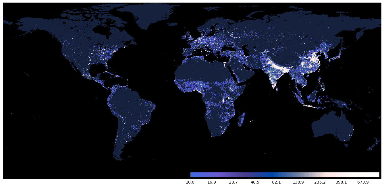
Global Mosaics 2000 - 2020 with a resolution of 1km
1
2
3
| DataPath = os.path.join(BasePath, 'unconstrained', '1km', 'global')
DataContents = os.listdir(DataPath)
print(DataContents)
|
1
| ['ppp_2020_1km_Aggregated.tif', 'ppp_2019_1km_Aggregated.tif', 'ppp_2018_1km_Aggregated.tif', 'ppp_2017_1km_Aggregated.tif', 'ppp_2000_1km_Aggregated.tif']
|
1
2
3
4
5
| Tifs = []
for i, file in enumerate(DataContents[:1]):
Tifs.append(gdal.Open(os.path.join(DataPath, file)))
print(f"{file:=^60}")
AboutTif(Tifs[i])
|
1
2
3
4
5
6
7
8
9
10
| ================ppp_2020_1km_Aggregated.tif=================
※ Number of bands: 1
--------------------
※ Raster size: 18720 rows x 43200 columns
-----------------------------------------
++++++++++++++ For 1 band +++++++++++++++
Null value: -3.4028234663852886e+38
Mean: 17.507 / SD: 240.278 / min: 0.000 / max: 53477.223
+++++++++++++++++++++++++++++++++++++++++
|
1
2
3
| band_data = Tifs[1].GetRasterBand(1)
nullval = band_data.GetNoDataValue()
img = band_data.ReadAsArray()
|
1
2
3
4
5
6
7
| cmap = mpl.colors.LinearSegmentedColormap.from_list("", ['royalblue', 'slateblue', 'darkslateblue', '#0047AB', '#6d809f', 'mistyrose', 'snow', 'white'])
logbounds = np.logspace(np.log10(10), np.log10(1e3), 71) # Note that I freely selected the value range for visualization.
norm = mpl.colors.BoundaryNorm(logbounds, cmap.N)
cmap.set_under('black')
cmap.set_bad(color='#16213E')
cmap.set_over(color='#FFC7C7')
cmap
|
1
2
3
4
5
6
7
8
9
10
11
12
13
| # set the color as a bad(np.nan) color in colorbar
img[np.logical_and(img >= 0, img < 10)] = np.nan
fig, ax = plt.subplots(facecolor='w', figsize=(17, 8))
# aspect의 디폴트값은 equal임. 입력된 array 크기로 figure가 forcing 됨.
im = ax.imshow(img, cmap=cmap, norm=norm, interpolation='none', aspect='auto')
ax.axis('off')
cb_ax = inset_axes(ax, width="50%", height="3%", loc='lower right')
fig.colorbar(im, cax=cb_ax, orientation='horizontal')
plt.show()
|
Take-Home Message and Discussion
- 이번 글에선 영국 사우샘프턴 대학 산하의 연구 그룹 “WorldPop”의 열린데이터 광장인 WorldPop Hub에서 Population Counts 데이터들을 들여다 보았다.
- 배포 중인 데이터들은 .tif 포맷이고, 이는 Raster (Gridded) 형태의 데이터를 의미한다.
- 각 그리드에는 Estimated of Population 값이 담겨있다.
- 각 국의 행정단위 상 Census 데이터를 그리드로 맵핑시키기 위해서 본 연구그룹은 Random Forest(RF) Mapping 방식을 적용했다.
- 거의 전세계 주요 개별 국가에 대해 Population Counts 데이터셋이 존재한다.
- UN Adjusted Postfix 가 붙은 데이터는 인구맵핑(with RF) 추정을 할 때, UN의 전세계 인구조사 결과를 반영해서 Correction을 한 데이터다. 이왕이면 이 데이터를 활용하기로 하자.
- Population Counts 데이터셋은 크게 ‘Unconstrained’ 버전과 ‘Constrained’ 버전으로 나뉘어져 있다.
- Unconstrained 은 Constrained 보다는 그리드에 추정된 인구수가 부정확하지만, 2000년부터 2020년까지 총 20개년의 데이터셋을 이용할 수 있다는 장점이 있다.
- Constrained 는 실제 Building Footprint 란 건물정보 메타데이터를 첨가하여 맵핑하였기에 더욱 정확하다는 장점이 있다. 다만 현재 가용데이터는 2020년 뿐이다.
- Unconstrained은 100m by 100m 또는 1km by 1km grid resolution 이 이용 가능하고, Constrained는 100m by 100m resolution만 이용 가능하다.
- Unconstraiend에는 개별 국가의 100m by 100m resolution을 이어붙여 만든 1km by 1km resolution의 Global(World) 스케일 Population 데이터도 함께 배포 중이다.
- 본 글에서는 우리나라(KOR)에 대해 100m 스케일의 Unconstrained(2002, 2008, 2014, 2020) 과 Constrained(2020) 데이터를 살피고 시각화해 보았다.
- 마지막엔 Unconstrained 1km scaled World Population Counts 2020 데이터도 살피고 시각화해 보았다.
fin